
Counter-Rotating Open Rotors performance evaluation
Performance for Contra-Rotating Open Rotors
Parameters
- base:
Base The base must contain:
the axial forces (‘flux_rou’ and ‘torque_rou’)
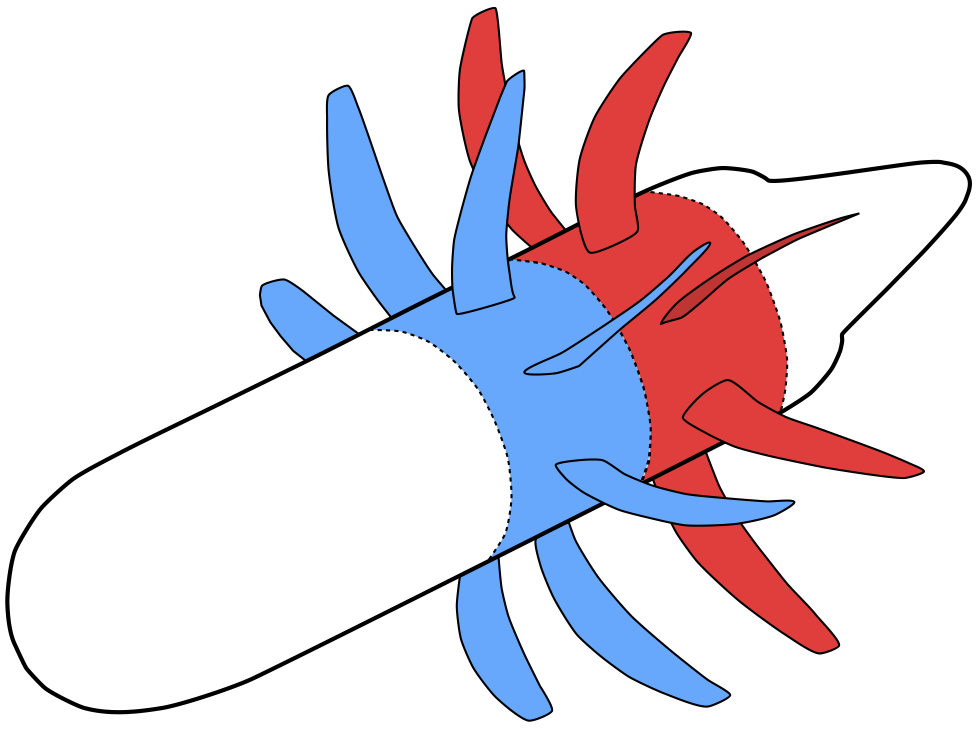
two zones, ‘front’ and ‘rear’, to separate the contribution from each rotor
‘nb_blade’ as an
Base.attrs‘n’ the rotation frequency as an
Base.attrs‘D’ the rotor diameter as an
Base.attrs.
- base:
- rho_inf: float
Infinite density.
- v_inf: float
Infinite velocity.
- duplication: bool, default= True
Duplication (rotation) of the forces. If not, for each row, the coefficients represent the forces, acting on a single blade, multiplied by the number of blades.
Main functions
- class antares.treatment.turbomachine.TreatmentCRORPerfo.TreatmentCRORPerfo
- execute()
Compute the similarity coefficients (forces) for a CROR. It is assumed that the forces come from a single canal computation (periodic or chorochronic when using HB/TSM approach). The forces are then duplicated by the number of blades.
Four coefficients are computed: the traction defined as
\(\displaystyle C_t = |\frac{flux\_rou}{rho\_inf \cdot n^2 \cdot D^4}|\),
the power coefficient defined as
\(\displaystyle C_p = |\frac{2 \pi \cdot torque\_rou}{rho\_inf \cdot n^2 \cdot D^5}|\) (note the simplification of the rotation frequency on the expression of the power coefficient),
the propulsive efficiency computed from the traction and the power coefficients
\(\displaystyle \eta = J \frac{C_t}{C_p}\), where \(J\) is the advance ratio defined as \(\displaystyle J = |\frac{v\_inf}{n \cdot D}|\) (note that this widely used formulation for propeller might be reconsidered in presence of a second propeller. Indeed, the second rotor “doesn’t see” the speed \(v\_inf\)),
and the figure of merit
\(\displaystyle FM = \sqrt{\frac{2}{\pi}}\frac{C_t^{3/2}}{C_p}\)
These formulae are computed rotor per rotor. The global performance is evaluated as follow:
\(\displaystyle C_t^{global} = C_t^{front} + C_t^{rear}\),
\(\displaystyle C_p^{global} = C_p^{front} + C_p^{rear}\),
\(\displaystyle \eta^{global} = \frac{J^{front} \cdot C_t^{front} + J^{rear} \cdot C_t^{rear}}{C_p^{global}}\)
\(\displaystyle FM^{global} = \sqrt{\frac{2}{\pi}}\frac{(C_t^{global})^{3/2}}{C_p^{global}}\)
- Returns:
the input base with the forces, a new zone ‘global’, and as many instants as the input base has. If the input base comes from a HB/TSM computation, the mean, and the harmonics are also computed. Note that the amplitude of the harmonics are given divided by the mean value.