The RTE (Eq.![[*]](icons/crossref.png) ) is solved for every discrete direction
) is solved for every discrete direction
 using a finite volume approach. The integration of the RTE over the volume
  of an element limited by a surface
  , and the application of the divergence theorem yields:
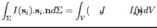 |
(1.3) |
The domain is discretized in three-dimensional control volumes
. It is assumed that  and
and
 are constant over the volume
and that the intensities
are constant over the volume
and that the intensities  at the faces are constant over each face. Considering that
is the averaged intensity over the
at the faces are constant over each face. Considering that
is the averaged intensity over the  face, associated with the center of the corresponding face, that
  and
and  are the averaged intensities over the volume
, associated with the center of the cell, and assuming plane faces and vertices linked by straight lines, Eq.() can be discretized as follows :
are the averaged intensities over the volume
, associated with the center of the cell, and assuming plane faces and vertices linked by straight lines, Eq.() can be discretized as follows :
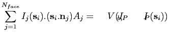 |
(1.4) |
where
 is the outer unit normal vector of the surface
  .
.
The scalar product of the  discrete
direction vector with the normal vector of the
face of the considered
cell is defined by
discrete
direction vector with the normal vector of the
face of the considered
cell is defined by  :
:
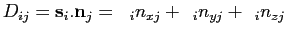 |
(1.5) |
The discretization of the boundary condition (Eq.()) is straightforward:
 |
(1.6) |
For each cell, the incident radiation  is evaluated as follows:
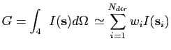 |
(1.7) |
and the incident heat flux  at the wall surfaces is :
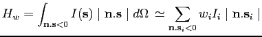 |
(1.8) |
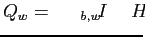
For a gray medium, the radiative source term  is given by:
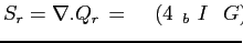 |
(1.9) |
where  is the radiative heat flux, and the radiative net heat flux at the wall is:
 |
(1.10) |
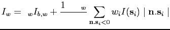
For the evaluation of the radiative intensity
in Eq. () to () Ströhle et al. [#!Str01!#] proposed a simple spatial differencing scheme based on the mean flux scheme that proved to be very efficient in the case of hybrid grids. This scheme relies on the following formulation:
 |
(1.11) |
where
 and
and
 are respectively the intensities averaged over the entering and the exit faces of the considered cell.
 is a weighting number between 0
and
is a weighting number between 0
and  . Substituting
from Eq.() into Eq.() yields (for more details see [#!IJTS!#]):
. Substituting
from Eq.() into Eq.() yields (for more details see [#!IJTS!#]):
 |
(1.12) |
The case  corresponds to the Step scheme used by Liu et al. [#!Liu00c!#]. The case
 is called Diamond Mean Flux Scheme (DMFS) which is formally more accurate than the Step scheme. After calculation of
from Eq.(), the radiation intensities at cell faces such that
is called Diamond Mean Flux Scheme (DMFS) which is formally more accurate than the Step scheme. After calculation of
from Eq.(), the radiation intensities at cell faces such that  are set equal to
, obtained from Eq.(). For a given discrete direction, each face of each cell is placed either upstream or downstream of the considered cell center (a face parallel to the considered discrete direction plays no role). The control volumes are treated following a sweeping order such as the radiation intensities at upstream cell faces are known. This order depends on the discrete direction under
consideration. An algorithm for the optimization of the sweeping order has been implemented [#!IJTS!#]. Note that this sweeping order is stored for each
discrete direction, and only depends on the chosen grid and the angular quadrature, i.e. it is independent on the physical parameters or the flow and may be calculated only once, prior to the full computation.
are set equal to
, obtained from Eq.(). For a given discrete direction, each face of each cell is placed either upstream or downstream of the considered cell center (a face parallel to the considered discrete direction plays no role). The control volumes are treated following a sweeping order such as the radiation intensities at upstream cell faces are known. This order depends on the discrete direction under
consideration. An algorithm for the optimization of the sweeping order has been implemented [#!IJTS!#]. Note that this sweeping order is stored for each
discrete direction, and only depends on the chosen grid and the angular quadrature, i.e. it is independent on the physical parameters or the flow and may be calculated only once, prior to the full computation.
Damien Poitou
2010-06-10