Tags :
- open_source: pypi, gitlab.com, readthedocs
- tool: Helper to setup a secured chain of jobs on a Job Scheduler
- CFD: Useful for all CFD runs to get statistics on users habits and machine usage
- Python package: available on pypi
- Excellerat: Relative to the task WP7.2 of the initial project: Making chained jobs easier for production runs by engineers
RUNCRAWLER, a tool for parsing your run folders and get statistics
Parallel computing programs such as CFD-solvers are often run on different machines, different geometries. Runcrawler is an open-source tool that can parse your run folder and give:
-
a big picture of what runs are done,
-
statistics on error logs of the code and what common mistakes done by users lead to the same mistakes or makes the code crash
Imagine you have a tool that can help you in a few graphs spot the loopholes of your team, in a few clicks, get to know who is not updating the code when they should, what recurrent mistakes make the code crash and burn a lot of CPU hours for nothing!
Maybe now is time to know if you should train the team some more, or make some changes in the code to avoid the same traps ever and after!
Depending if you are an end user, a HPC expert, or just the big boss of a team playing with several codes on several clusters, this tool will give you some precious information about users’ good and bad habits, code traps, and some HPC tricks that might need some highlighting fo users.
Each company has HPC experts able to tell how many hours users burnt on clusters, whether they are inside the company or remote. This information is needed to track accountance but also to prepare demands for more hours by the suppliers. Each year, billions of burnt hours lead to a few papers produced by the team, with an undeniable added value in the scientific field. And what if we were able to draw the actual link between a paper and CPU hours burnt for it, for example if scientific advance was made on a specific model, we want to know which CPU hours were run on this model, or for a specific geometry, if we identify a combustion chamber by a specific number of cells, we will be able to say which CPU hours are linked to this mesh in particular.
How it works
Runcrawler is an open source tool which can be simply installed. After you will just have to specify the path for data to mine in a python module called runcrawler.py. This python module creates a database of json files that are then collected by a jupyter notebook that parses the json files. It creates a pandas dataframe where each line corresponds to a run.
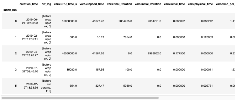
A pandas dataframe is also a nice representation of big data and you can get a quick overview of the data just by calling the function .head(). The columns of the dataframe are all the parameters we know about the runs such as the user, the date, the version of the code used, the time elapsed, all the physical parameters or geometrical parameters such as mesh size.
The jupyter notebook performs some data pre-treatment to get rid of NaN values so that it is then fully ready for statistics. A lot of graphical representations are easy and quick to get by using the built in python library Seaborn or simply just the built-in graphical functions of pandas.
Parsing the runs and get statistics
Here we will look at how we can get some useful information out of a database or runs of a team looking at three aspects: - the adoption percentage of new version of codes - the error logs - HPC data such as the code efficiency and parallelization habits.
AVBP Statistics
User’s habits
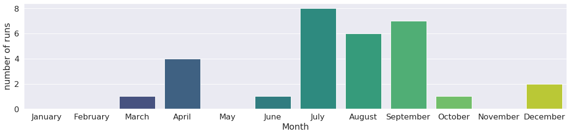
We can track what days of the week most of the runs were launched. This can be useful information for optimization of when week and weekend machine queues are used. This user has a tendency of launching runs on tuesdays and wednesdays as the histogram below shows !
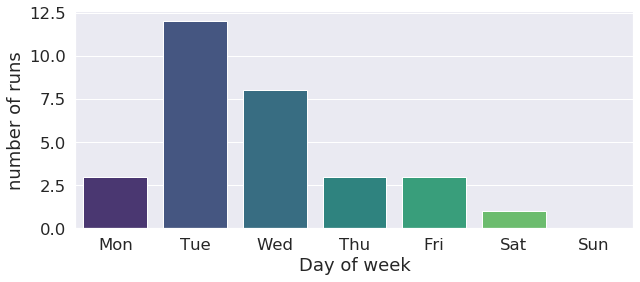
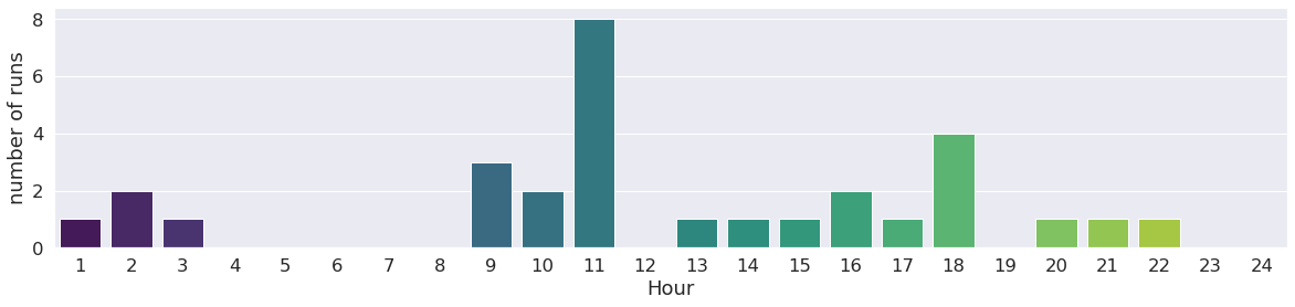
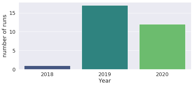
We can go further with this investigation by classify runs by year, month, hour too !
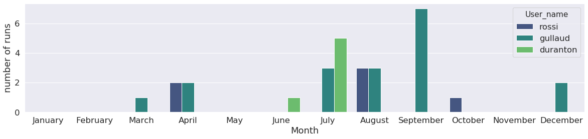
Runs can also be classified by user:
Statistics on what kind of run was launched
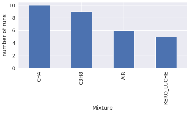
Mixture
The first graph shows that most of the runs were conducted with methane (CH4), followed by propane (C3H8).
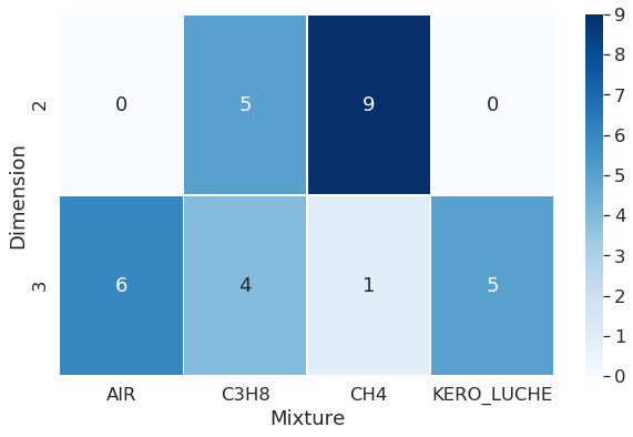
All mixtures were tested on 3D geometries, whilst only two type of mixtures were tested on 2D dimension geometries.
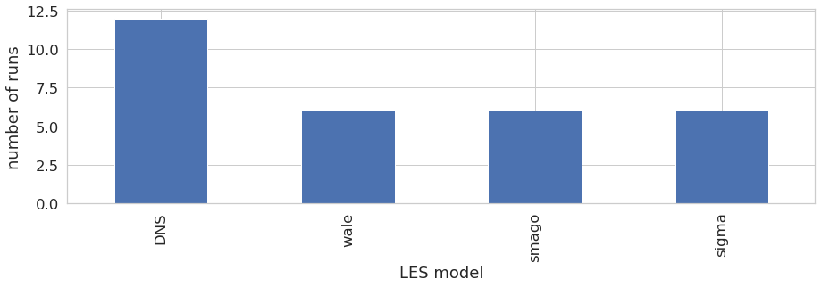
LES model
The Large-Eddy Simulation (LES) code AVBP offers several choices for the LES model, here we can see that the user performed 16 runs using the WALE les mode, 8 runs with the LES model from Smagorinsky, 3 with the sigma model, and 13 wihout models, which means DNS (Direct Numerical Simulation) was performed.
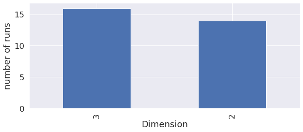
Dimension
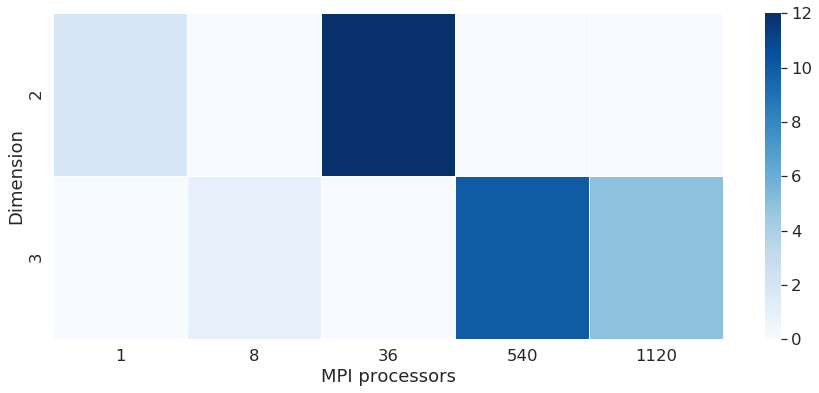
AVBP is able to perform 2D or 3D runs, but sometimes, 2D results cannot give as much precision as 3D runs, so it’s interesting to check that the user indeed performed 3D runs.
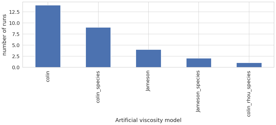
Artificial viscosity model
The classification on artifical viscosity model shows that the user tested all artificial viscosity model available, with a preference of Colin model.
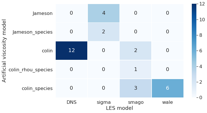
Combination of LES model and artificial viscosity model
This graph shows together the LES and artificial viscosity model chosen for the run. We can see that DNS was performed only with Colin. And the Jameson model was used only with the LES model called sigma.
High Parallel Computing (HPC) metrics: mesh nodes, Central Processing Unit (CPU) time, efficiency and scalability
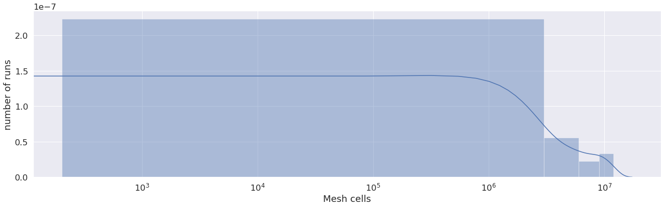
This graph shows an overview of the number of cells in each mesh used for the runs. We see in this case the user used from about 70 cells to 38 million cells, which is a high variety of runs.
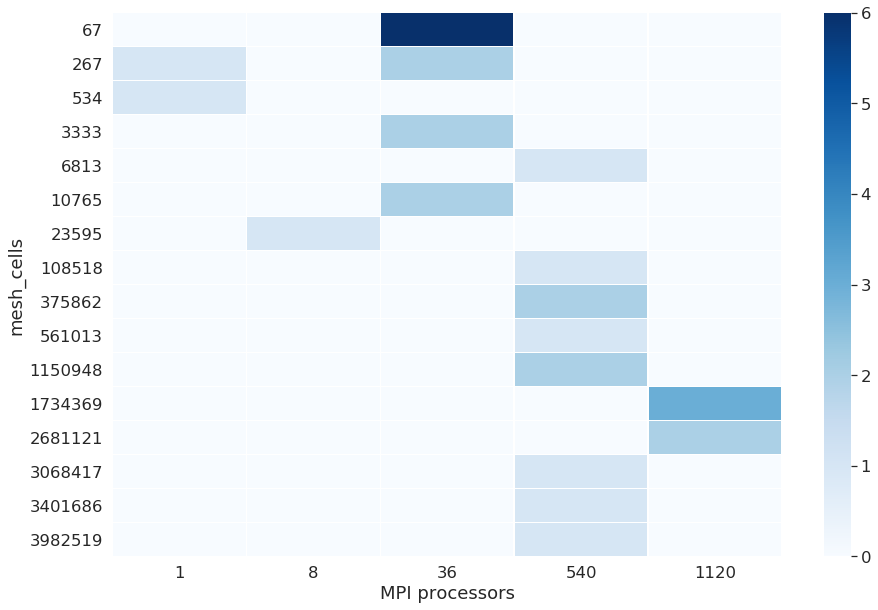
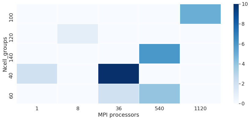
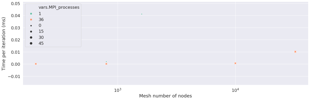
It will not be necessary for each mesh to parallelize the runs. The CPU parameters depend on the mesh. Here we show how many MPI (Message Passing Interface) processors the user used to run which run, depending on the number of nodes in the mesh. When the number of MPI processes is equal to 1, it means the runs was not parallelized, it is the case for a low number of cells, in this case, below a thousand. The following graphs show how much MPI processors were used depending on the mesh cells, and helps check if the user did the right thing parallelizing the runs. An HPC expert can help improve the runs by upgrading the number of cells in groups for each MPI run done.
We can see on some points the scalability of the machine. The scability is a metric used to explore the performance of codes. We have to see the behaviour of runs with the same number of cells scaled on a higher number of processors. We see here that the time per iteration decreases when we run the same number of cells on 1 processor or 36 processors. Note: the database for runs here is not sufficient to evaluate this metric in a proper way.
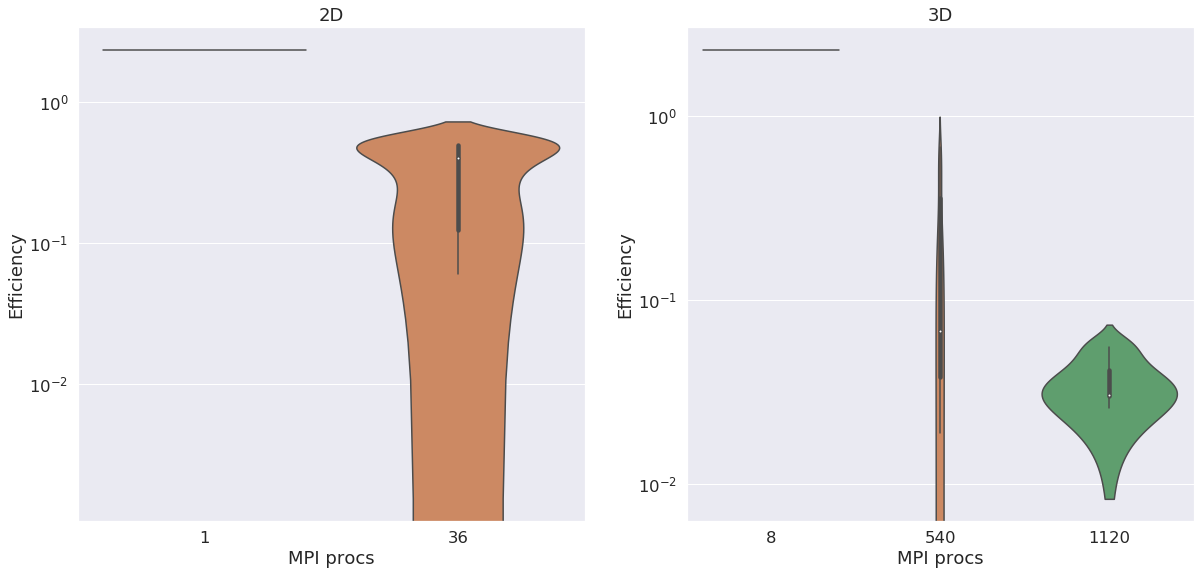
We compute the efficiency of the machine, which is defined by the time spent by one processor to compute one node of the mesh. This metric is used to compare machine performances. it is expressed in µs/ite/node. The figure below shows efficiency for 2D and 3D runs. We can see the efficiency gets better in both dimensions by raising the number of MPI processes.
Error logs
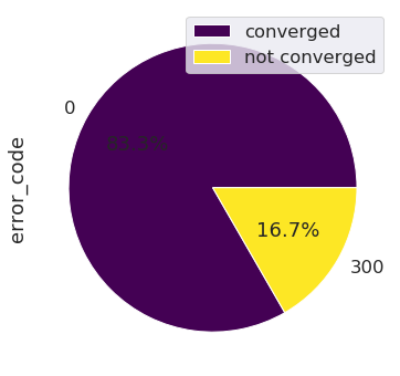
The number of runs is classified by error logs: In this case, for example runs went out with the 0 error log, which means no error occured, or a 300 error log, which correponds to an error occuring before the temporal loop occurs.
This chart pie shows the percentage of runs that are converged versus the runs that did not converge.
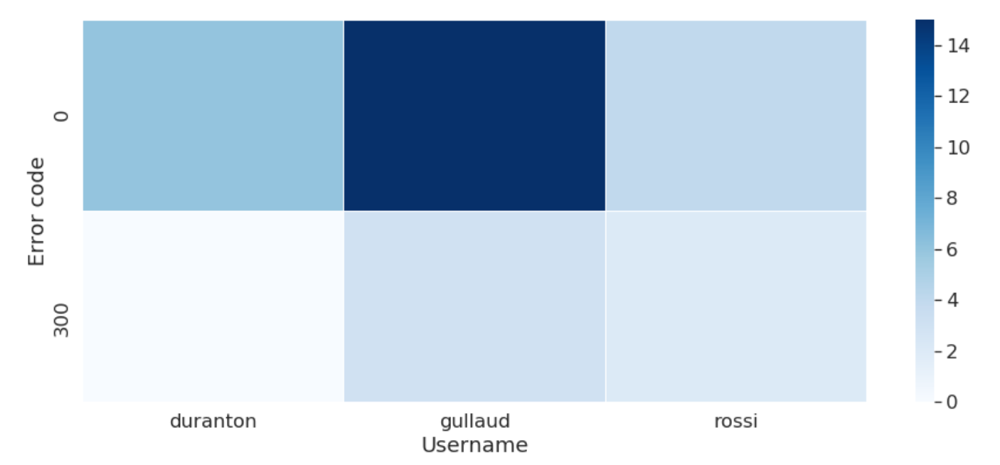
The tendency of errors linked to the user can also be visualized:
Clustering
We want to classify the runs by groups. First, we are going to look at the problem in an unsupervised manner, that means, not looking at the fact that a run is converged or not, we are just going to let the algorithm find properties of runs close to each other and create clusters out of it. The dimensions of our runs dataframe contains 26 features, that’s why we are first going to reduce the dimensions of these features. In a second step, we are going to make clustering on these reduced dimensions.
A well-known dimension reduction algorithm used with the library scikit-learn is Principal Component Analysis (PCA). PCA takes in a number of dimensions and is going to render vectors that are linear combinations of original features, features with the most important weight being the features that allow to keep the most standard deviation in the data.
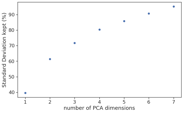
Dimensions of the PCA can be derived by plotting the standard deviation across the dimension. Here we see that we should have 4 dimensions in the PCA to keep 80% of the standard deviation.
To keep things as simple as possible, we are first going to perform PCA in a 2 dimension environment.
PCA in 2 dimensions
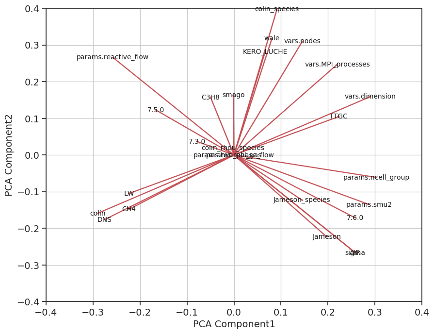
We perform PCA with 2 dimensions, that means that each run is going to be expressed in a 2D environment.
The two components of the PCA that are determined by the algorithm are a linear combination of the original features as shown in the DataFrame below. They can also be represented by a heatmap:

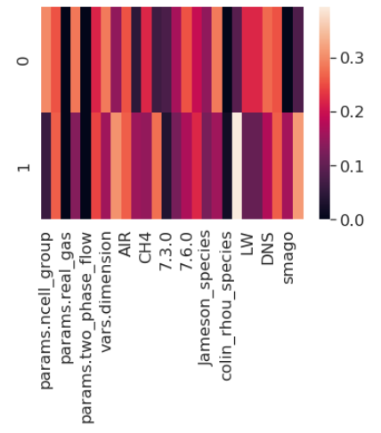
The representation of PCA components as vectors of the original features is a nice representation to see the weight of each feature. It is easy to see that PCA first component is equally weighing dimension and ncell_Group but not considering wale. On the other hand PCA second component has a bigger component of smago.
K-means clustering on the reduced dimension data
K-means is a clustering algorithm used for unsupervised learning. It is aiming at reducing the distance of each point to it’s cluster’s centroid, and creates separated groups of points having approximately the same euclidean distance to its center.
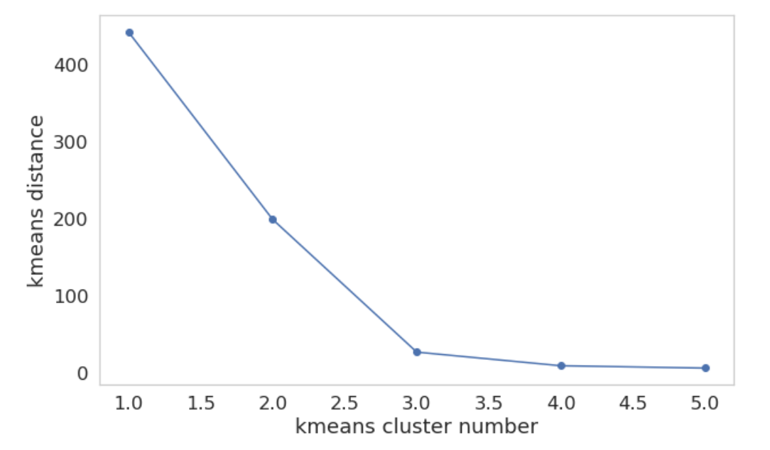
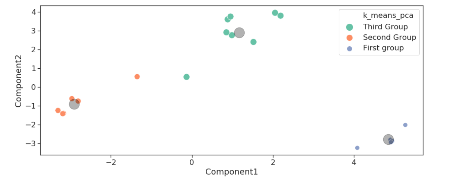
This graph shows the accumulated distance in each group depending on the number of clusters. We see that a number of 3 clusters is optimal. Beyond that number, the distance doesn’t decrease as much.
On this graph, we see three groups appear with their centroids in grey. On x and y are the two components of the PCA.
We can now look at the characteristics of the runs gathered in each group. Each feature that is giving the less standard deviation is proving to be the most important feature of the group.
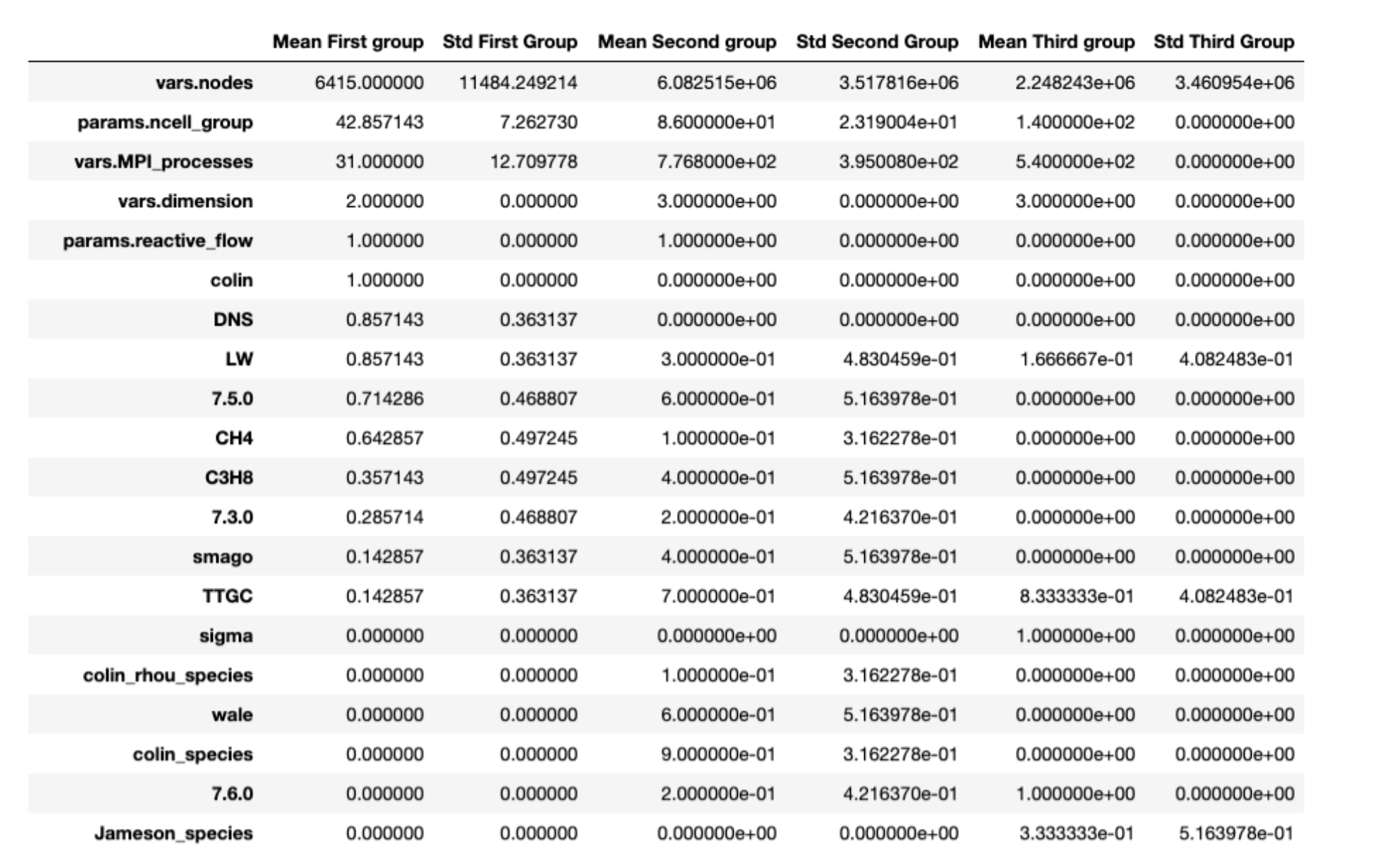
The third group is exclusively made of runs in 3D dimension, and run on 140 cells and 540 procs with only Air as a mixture.
On the other hand, the first group is only runs in 2D, with mesh cells much lower than other groups (the standard deviation being around 11k with a mean value around 6k whilst the other groups have a value around one million).
Conclusion and further work
We are going to look at this problem in a supervised way, see if there is a relationship between the clusters and the converged/non converged property. This study should be made on a much higher dataset of runs to prove its capability.
Runcrawler aims at given a better undestanding of traps leading to runs crashing. Playing with data already helped us identify some critical points in the database: - team players don’t really update the code version when they should, this way they tend to use bugged versions of the code, and are going to loose some precious time on bugs that have been resolved for sure, - Efficiency has a nice trend but outliers should be looked at! - Some HPC parameters such as ncgroups are not well used by some users.
A lot of parameters are associated with each run, so we are looking for methods which can help reduce dimension of data. Principal component analysis can help us identify the features that enter the most in action for making a run converge or crash. In our example that contains 28 columns, meaning features describing one run, PCA can help us identify 2 or more components that are linear combinations of the original features. That way we are able to represent our data in 2Ds or 3Ds, which would be impossible in 28 dimensions ! Read further on PCA and clustering in this further study.
This work has been supported by the EXCELLERAT project which has received funding from the European Union’s Horizon 2020 research and innovation programme under grant agreement No 823691.