Tags :
- HPC: High Performance Computing management
- Excellerat: Relative to the task WP7.2 Standardization
This is the worked example of the idea, read the rationale here.
Reading time: 15 min
A worked example of feedback process
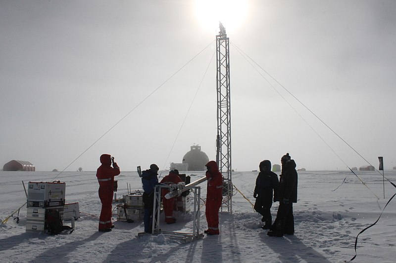 Ice core researchers drilling at the EastGRIP ice core site, Greenland. Can we learn about our simulations in a similar fashion?
Limits of accounting today
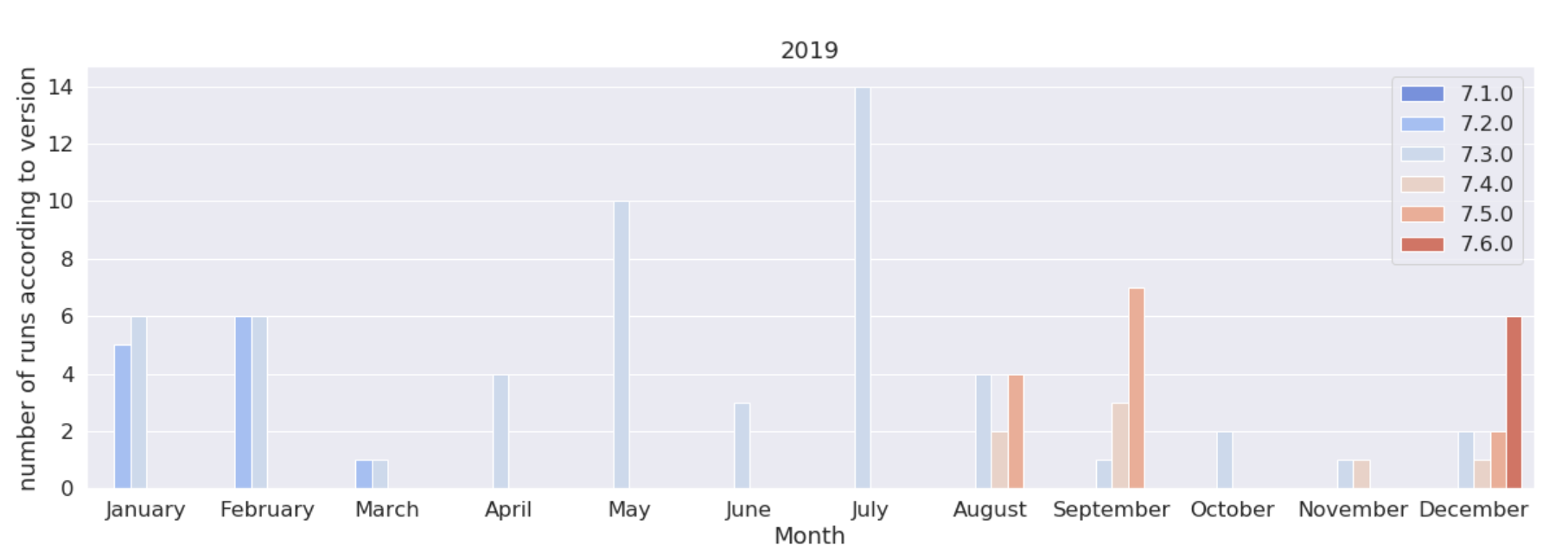
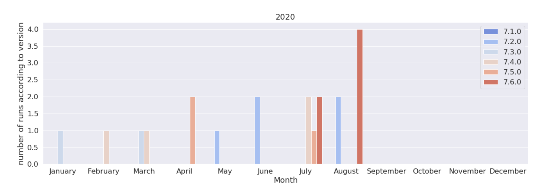
HPC clusters usually rely on batch submission software (e.g., Slurm), which offers a command line interface for users to request compute resources, and performs allocation of these resources according to the rules defined by the system administrator. Submission software include activity logs with the goal of billing CPU-hours according to each user’s consumption. The following figures give an overview of the distribution of consumption between users.
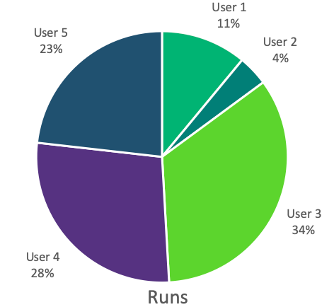
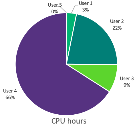
While CPU-hours are directly billed to the user, each run must be started by hand, hence the number of runs is an indication of the associated labor costs. Both of these metrics are therefore useful to assess the total simulation costs.
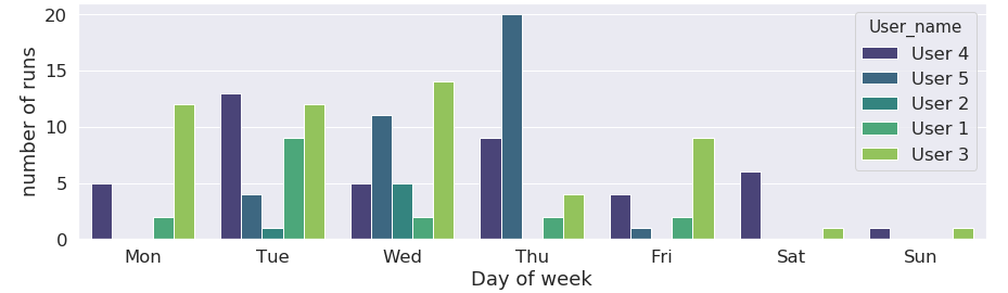
The data also reveals user habits, and can inform the system administrator to tune the job scheduling rules and improve productivity. In the following graphs, users have uneven usage patterns throughout the week.
Here is what accounting looks like practically. Queries are done on the jobs log, for example with a command line in the terminal of the machine:
>slurm-report.sh -S 090120 -E now -T -g cfd
In this case, the job scheduler is SLURM. The command slurm-report.sh gathers information from September 1st -S 090120 to today -E now for the users group cfd -g cfd. The output looks like this:
       JobID    JobName  Partition     Group    Account  AllocCPUS    Elapsed      User CPUTimeRAW
------------ ---------- ---------- --------- ---------- ---------- ---------- --------- ----------
401637             batc       prod       cfd    default         72   12:00:29     anonymous1    3112488
401643              lam       prod       cfd    default        540   12:00:22     anonymous1   23339880
401805         F53NTPID       prod       cfd    default        540   12:00:22     anonymous2   23339880
401808         F53A1NTP       prod       cfd    default        540   12:00:22     anonymous2   23339880
401813          OFCo706       prod       cfd    default        540   12:00:22     anonymous2   23339880
401815          OFCo530       prod       cfd    default        540   03:03:16     anonymous2    5937840
401837         A_STABLE       prod       cfd    default        540   07:54:25     anonymous6   15371100
401873             batc       prod       cfd    default         72   00:00:00     anonymous1          0
401875              lam       prod       cfd    default        540   00:00:00     anonymous1          0
401916        labs_lolo       prod  stg-elsa    default        540   00:04:16     anonymous3     138240
401999          NEW_TAK       prod       cfd    default        540   05:22:30     anonymous4   10449000
402004        Z08_URANS       prod      elsa    default        180   07:47:19     anonymous5    5047020
(...)
There are now groups and tools focused on extracting information from these use database. For example the UCit is developing a framework Analyse-IT based on data-science to explore the database. The database is gathering only the information the job scheduler is aware of. The typical job profile is, at best:
- Job name
- User login and group
- Account (if needed)
- Executable Name
- Queue (Nb of cores)
- Duration requested
- Memory requested
- Start and end time
- Exit code
The executable name, user-defined, is often not exploitable (e.g. /awesomepath/new_version.exe). The exit code must also be handled with care because no standard of exit codes exists for an HPC software.
The conclusion is therefore simple, there is neither engineering-related data nor software-related data under the watch of the job scheduler.
Where to find new information
The accounting database is not tracing engineering information: What are the engineering phenomenons taken into account, the size of the computations, the additional features, etc… These elements are forecast at the beginning of the year to size the CPU allocation requested. All the data is in the setup. The challenge is to gather it across all runs.
The accounting database is not tracing software information either: What was the version in use, the actual performances, the job crash origin, etc… The software is usually providing the answers through a log file, one per run. The same challenge appears : gathering the log files across all the runs.
Coring of simulation logs
The ideal solution would be to feed daily a dedicated database, like the accounting one. But designing a system, tackling permissions and confidentiality issues, defining common definitions on performances and crashes and many hurdles lie ahead. We will depict here a “brute force” approach to make some baby steps in this direction.
The simulations done by engineers for design are, usually, saved on archive disks. A large amount of the relevant setups and log files are still available at the end of the year. We can tap these disks to get a partial, but quantitative, overview of what was done.
Here follows extracts of a setup file and a log file for the Computationnal FLuid Dynamics solver AVBP. The input file run.params is a keyword-based ASCII file with several blocks depending on the complexity of the run.
$RUN-CONTROL
  solver_type = ns
  diffusion_scheme = FE_2delta
  simulation_end_iteration = 100000
  mixture_name = CH4-AIR-2S-CM2_FLAMMABLE
  reactive_flow  = yes
  combustion_model = TF
  equation_of_state = pg
  LES_model = wale
  (...)
$end_RUN-CONTROL

$OUTPUT-CONTROL
  save_solution = yes
  save_solution.iteration = 10000
  save_solution.name = ./SOLUT/solut
  save_solution.additional = minimum
  (...)
$end_OUTPUT-CONTROL

$INPUT-CONTROL
   (...)
$end_INPUT-CONTROL

$POSTPROC-CONTROL
    (...)
$end_POSTPROC-CONTROL
Most of the missing information about the configuration are present. However, due to the jargon, a translator is needed. For example, few people outside the AVBP users know that pgis the keyword for a perfect gas assumption.
Then comes the AVBP typical log file, presented hereafter, with sections cropped for readability.
Number of MPI processes :           20


     __      ______  _____   __      ________ ___
    /\ \    / /  _ \|  __ \  \ \    / /____  / _ \
   /  \ \  / /| |_) | |__) |  \ \  / /    / / | | |
  / /\ \ \/ / |  _ <|  ___/    \ \/ /    / /| | | |
 / ____ \  /  | |_) | |         \  /    / / | |_| |
/_/    \_\/   |____/|_|          \/    /_/ (_)___/


Using branch  : D7_0
Version date  : Mon Jan 5 22:03:30 2015 +0100
Last commit   : 9ae0dd172d8145496e8d62f8bd34f25ae2595956

Computation #1/1

AVBP version : 7.0 beta

(...)

 ----> Building dual graph
    >> generation took 0.118s

 ----> Decomposition library: pmetis
    >> Partitioning took  0.161s

       ___________________________________________________________________________________
       | Boundary patches (no reordering)                                                |
       |_________________________________________________________________________________|
       | Patch number   Patch name                         Boundary condition            |
       | ------------   ----------                         ------------------            |
       | 1              CanyonBottom                       INLET_FILM                    |
       (...)
       | 15             PerioRight                         PERIODIC_AXI                  |
       |_________________________________________________________________________________|

       _______________________________________________________________
       | Info on initial grid                                        |
       |_____________________________________________________________|
       | number of dimensions              : 3                       |
       | number of nodes                   : 34684                   |
       | number of cells                   : 177563                  |
       | number of cell per group          : 100                     |
       | number of boundary nodes          : 9436                    |
       | number of periodic nodes          : 2592                    |
       | number of axi-periodic nodes      : 0                       |
       | Type of axi-periodicity           : 3D                      |
       |_____________________________________________________________|
       | After partitioning                                          |
       |_____________________________________________________________|
       | number of nodes                   : 40538                   |
       | extra nodes due to partitioning   : 5854 [+  16.88‰]        |
       |_____________________________________________________________|

(...)

 ----> Starts the temporal loop.

       Iteration #      Time-step [s]         Total time [s]        Iter/sec [s-1]

                1    0.515455426286E-06    0.515455426286E-06    0.357797003731E+01
             ---> Storing isosurface: isoT
               50    0.517183938876E-06    0.258723148413E-04    0.184026441956E+02
              100    0.510691871555E-06    0.515103318496E-04    0.241920225176E+02
              150    0.517872233906E-06    0.772251848978E-04    0.239538511163E+02
              200    0.523273983650E-06    0.103271506216E-03    0.241928988318E+02
              (...)
            27296    0.547339278850E-06    0.150002454353E-01    0.241129046630E+02

 ----> Solution stored in file : ./SOLUT/solut_00000007_end.h5

             ---> Storing cut: sliceX
             ---> Storing cut: cylinder
             ---> Storing isosurface: isoT

 (...)

 ----> End computation.

 ________________________________________________________________________________________________________

       _____________________________________________________________________________________________
       | 20 MPI tasks             Elapsed real time [s]       [s.cores]      [h.cores]             |
       |___________________________________________________________________________________________|
       | AVBP                   :      1137.27               0.2275E+05     0.6318E+01             |
       | Temporal loop          :      1134.31               0.2269E+05     0.6302E+01             |
       | Per iteration          :       0.0416               0.8311E+00                            |
       | Per iteration and node :   0.1198E-05               0.2396E-04                            |
       | Per iteration and cell :   0.2340E-06               0.4681E-05                            |
       |___________________________________________________________________________________________|


 ----> End of AVBP session


 ***** Maximum memory used : 12922716 B ( 0.123241E+02 MB)
Here again, a lot of information is present : version number, performances indicators, problem size, etc…
The cause of crashes is still missing. However, there is a way out because log files are written in chronological order.
| If the log file stops before: | the error code is: | Which means: |
|---|---|---|
Input files read |
100 | Ascii input failure |
Initial solution read. |
200 | Binary input failure |
Partitioning took. |
300 | Partitioning failure |
----> Starts the temporal loop. |
400 | Pre-treatment failure |
----> End computation. |
500 | Temporal loop failure |
----> End of AVBP session. |
600 | Wrap up failure |
| all flags reached | 000 | Success |
These error codes can be code-independent. However, one can increase the granularity of the error codes by adding code-dependent custom error codes.
For example in AVBP, a thermodynamic equilibrium problem is raised by the error message Error in temperature.F which can return a specific code (e.g. 530) to keep track of this particular outcome in the temporal loop.
Gathering the data.
In this brute force approach, a script, the “crawler”, is run on the filesystem complying to the Unix permissions. This data-mining step, can take some time. Here is a rough description of the actions used for this illustration:
- First search for the log files , and discard duplicates with a checksum comparison.
- Find the corresponding setup file.
- Parse the log file with regular expressions (regexps) and compute the error code.
- Parse the setup file, again with regexps.
- Keep that of the creation date and the login of the creator
- File this data into a database.
The final database is then filled with both pre-run information (the setup, version time, and username) and post-run information (error codes, performances, completion).
Remember the two limits of this approach:
-
this database will not take into account runs erased during cleanup operations. It cannot be considered exhaustive, unless the crawler is run regularly with a scheduler like a crontab.
-
all runs are equally represented (with an equal interest). In reality only one out of ten runs, at best, is actually contributing to a motivated engineering conclusion. Some runs are only taken to check to versions of the same code give similar results. The added value of a specific run, compared to another, is subjective.
There is however a nice database to investigate…
Quantify the crashes
Software support is the elephant in the room taking most of the time but never mentioned. We were talking about reducing the stress on the support team, maybe we can help them to target the weakest points of the code?
This pie chart highlights the percentage of runs that went through and those which crashed, due to different errors. An error code of ‘0’ indicates a run that went through. Any other error code means it crashed.
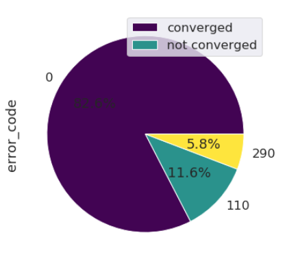
Here we see that almost 12% of the runs crash due to an error code of ‘110’ which means bad filling of the input file. The CPU hours are not wasted, but the end-user hours are, and this builds resentment. Various ideas could pop :
- maybe the parser is too strict?
- or the documentation could be improved?
- Could it be that some dialogs are giving the wrong mental model?
Here the support team should not give in to the temptation to guess. With the new database, one can focus on the runs that crashed and get new insights, either by manual browsing, or a new data-science analysis if there are too many.

Actual versus expected performance
The HPC pledge : my code is faster on a higher number of processors. On a priori benchmarks with controlled test case, the figures are nice and clean. What about an a posteriori survey on the past batch of simulations?
Efficiency, the time needed to advance one iteration (a computation step), divided by the number of degrees of freedom (the size of the mesh), is used to compare machine performances. Units are µs/iteration/degree of freedom.
Important, efficiency comparisons between two different codes are deceptions: the iteration is a code-specific concept, and the d.o.f. quantity can be difficult to convert.
In one way or another, efficiency must linearly decrease with the number of cores .
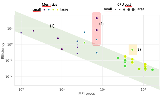
We can see the linear trend with the number of MPI processes. This overall trend is right. Unfortunately, there are terrible outliers : 2 orders of magnitude slower on the same code and same machine cannot not be taken lightly. A special investigation should focus on this.
If we dig further in the code-dependent figures, the cache of AVBP can be optimized with the ncell_group parameter. As this is configuration dependent and features dependent, the process of finding the right tuning has always been heuristic. Here we look at a heat-map of the ncell_group parameter versus MPI processors to go even further and check if the association of both parameters is right.
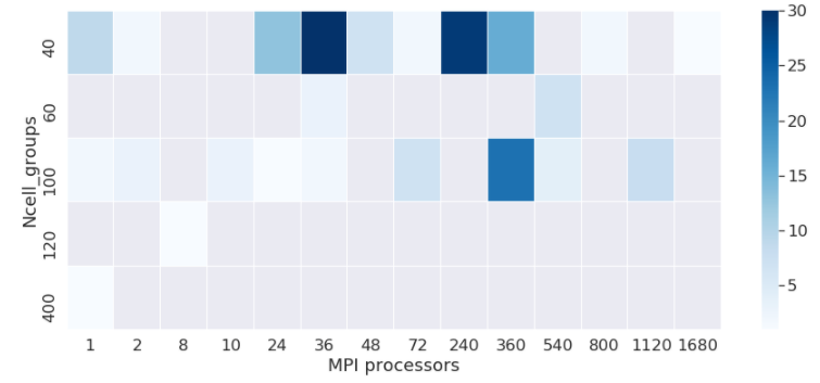
ncell_group is tested by the user to improve their simulations on the partitions.
The fact that only 5 values are found is the proof very few people take the time to optimize the cache with respect to their simulation.
Version acceptation
HPC users can exhibit a lot of inertia in their version upgrades. Here we will track the adoption rate of new versions among users.
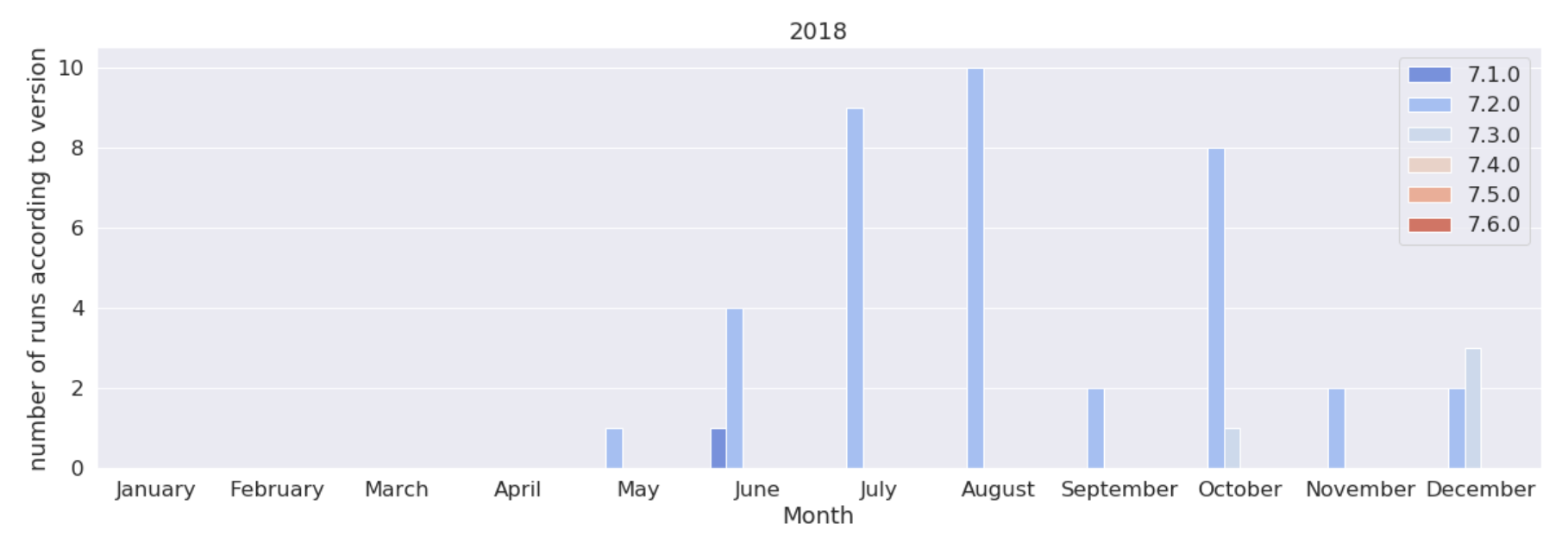
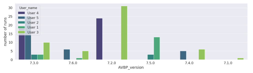
The popularity figure shows that user 2 and 4 never moved to the 7.6 version. User 4 stayed limited to the 7.3 version, while using 66% of the CPU hours.
Sorting families of simulations
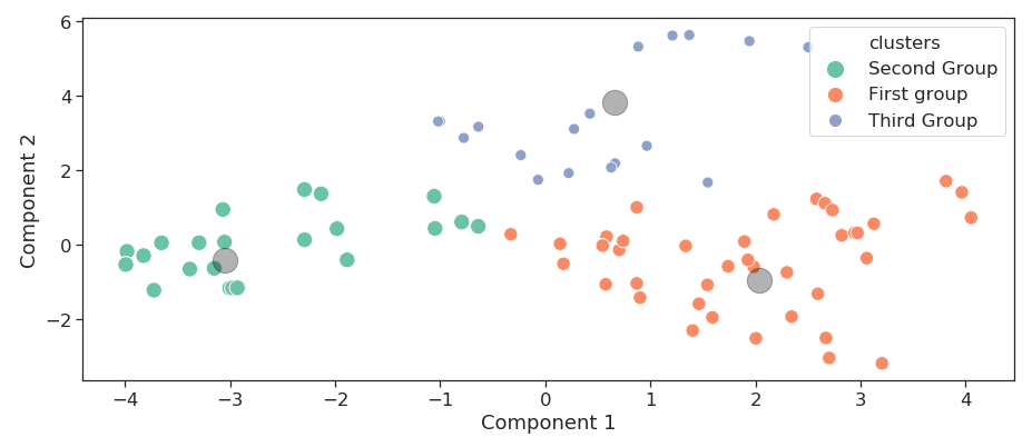
Sorting is a machine learning task. Principal Component Analysis (PCA) reduce dimensions of data. It brings down a lot of components to a 2, 3, or 4 major components, while keeping the same diversity.
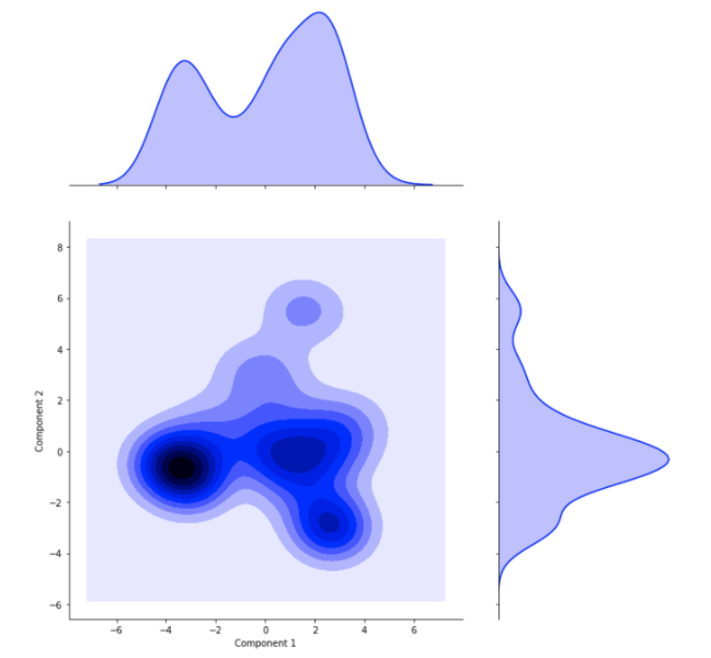
PCA gives simpler representation of the variability on the database, but no clue about what are these emerging clusters. We can gather groups of similar runs thanks to clustering. We see in the following 2-components scatter plot that runs have been automatically separated into three groups that have close parameters. This way runs can be sorted without human supervision and bias.
Finally the initial components of the database are compared between the clustered families. A prominent component is therefore a specific trait of a family.
- numerical aspects
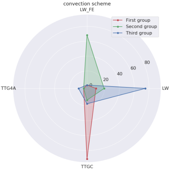
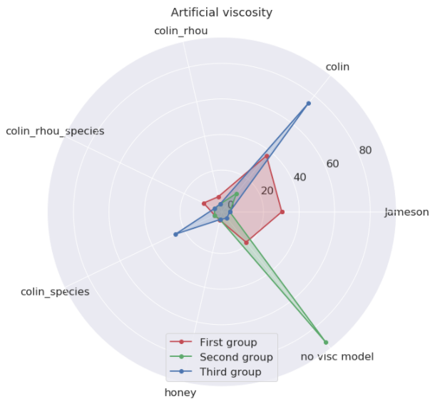
The three families are compared on two numerical aspects. The convection scheme used is a striking deference between the three. The numerical viscosity choice is also opposing the second and third group.
- Flow modeling
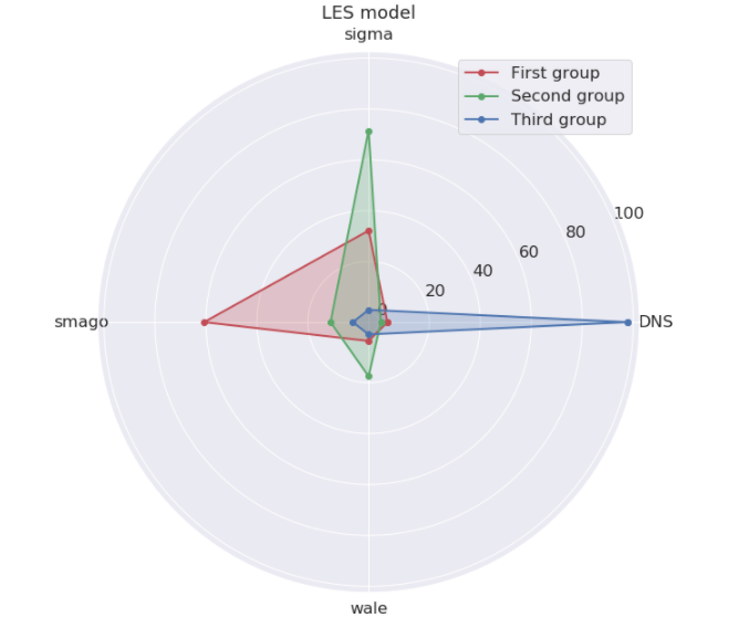
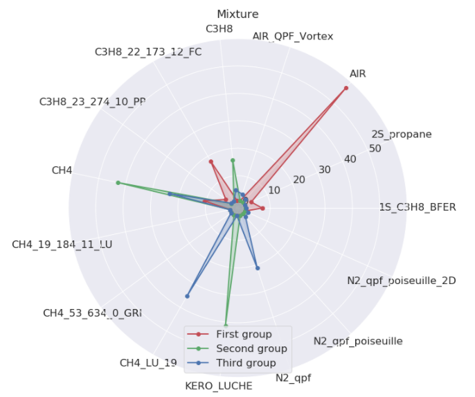
The LES model is a fluid turbulence modeling. Again the three families use different modeling strategy.
(DNS means no model was used). The mixture name is the gas composition in use. Here no mixture is a unique trait for any families (AIR is the oxygen-nitrogen cocktail, KERO, C3H8 and CH4 are usual fuels. Other mixtures are for test purpose (*_qpf_*) or higher precision fuel kinetics (fuel)-_(n_specs)_(n_reac)*.)
This “family profiling” give the following insight:
- The largest family is about non-reactive (AIR) configurations done with high order schemes (TTGC).
- The second family is the reactive runs with classic fuels (KERO, CH4, C3H8) with normal finite elements schemes (LW-FE). Surprisingly for an expert of AVBP, there is often no artificial viscosity, but a complex LES model (Sigma).
- The last group from clustering analysis is usually harder to profile. The third family is done with a normal scheme (LW) and no LES model, therefore laminar flow with no need of precision on the convection.
Drawback of the method
When applying these approaches, one should keep the Mc Namara Fallacy in mind, detailed by D. Yankelovich:
The first step is to measure whatever can be easily measured. This is OK as far as it goes. The second step is to disregard that which can’t be easily measured or to give it an arbitrary quantitative value. This is artificial and misleading. The third step is to presume that what can’t be measured easily really isn’t important. This is blindness. The fourth step is to say that what can’t be easily measured really doesn’t exist. This is suicide. — Daniel Yankelovich, “Corporate Priorities: A continuing study of the new demands on business” (1972).
Until today, there was no strong incentive for a quantitative monitoring of the HPC industrial production in terms of phenomenon simulated, crashes encountered, or bad user habits. Those were not quantifiable and usually disregarded. If we add this kind of monitoring to the HPC toolbox more largely, we could also open a production hell where the monitoring metrics will become new additional constraints. By the means of the Goodhart’s law, the production quality could worsen even under this new monitoring. We would have quit one fallacy just to stumble into an other one. If such initiative became a new layer of additional work, this would be a backfire : the mindset of the work presented here is to reduce the work, the stress and the waste of both human and hardware resources.
In a nutshell
This worked example showed how to core information in the former jobs logs.
- A crawler explores the disks to find logs, and parses both the input and log files to feed a database.
- A specific process analyses the log file to provide error codes if these files are interrupted before a nominal end.
- Errors, version acceptation, and actual performances can be monitored from this database.
- The batch of simulations can be sorted in main families. First, run a Principal Component Analysis to reduce the complexity of the database. Second use clustering to gather jobs into families. Finally find the unique traits of families until these groups are making sense.
The tools used for this worked example should quickly be released as open-source tools from the CoE Excellerat under the name of runcrawler.
Acknowledgements
This work has been supported by the EXCELLERAT project which has received funding from the European Union’s Horizon 2020 research and innovation program under grant agreement No 823691.
![]()
The authors wish to thank M. Nicolas Monnier, head of CERFACS Computer Support Group for his cooperation and discussions, Corentin Lapeyre, data-science expert, who created our first “all-queries MongoDb crawler”, and Tamon Nakano, Computer science and data-science engineer who followed-up and created the crawler used to build the database behind these figures. (Many thanks in advance to the multiple proof-readers from the EXCELLERAT initiative, of course)