Disclaimer : under construction
Tags :
- open_source : pypi, gitlab.com, readthedocs.
- CFD : 2 CFD solvers, one Navier-Stokes, one Lattice Boltzmann.
- training : dedicated to CFD training.
- Python package : available on pypi.
Barbatruc - Finite Differences Navier-Stokes and LBM for CFD training.
Barbatruc is a package for Computational Fluid Dynamics (CFD) trainings. This repository is education-oriented and illustrates the principle of dependency inversion for CFD-solvers. It becamed a side product of the EXCELLERAT Center of Excellence project, funded by the EU.
There are three basic cases developed in barbatruc: a poiseuille 2D flow, a lid-driven cavity flow and a flow around a cylinder. Each one of these examples has a simplified data-structure for a cartesian, regular i-j mesh. The solvers must fit into this datastructure, without interferring.
For each case, a time loop is used to solve it, the setup is as follow:
Finite differences forward explicit solver for Navier-Stokes
solver = NS_fd_2D_explicit(dom, max_vel=2*vel)
for i in range(nsave):
    time += time_step
    solver.iteration(time, time_step)
    print("\n\n===============================")
    print(f"\n  Iteration {i+1}, Time :, {time}s")
    print(f"  Reynolds : {dom.reynolds(width)}")
    print(dom.fields_stats())
    dom.dump_paraview(time=time)
By the end of 2019, two solvers are implemented with the same signature :
-
Explicit finite difference solver, rewritten from Lorena Barba, in 200 lines.
-
Lattice Boltzmann 2DQ9 solver, in 400 lines.
Be aware that the Lattice Boltzmann solver (LBM) is not ready for release yet.
Poiseuille
This is the simplest case you can find in barbatruc.
There are two cases for Poiseuille.
First case:
It consists of periodic boundary conditions as input and output, and no slip conditions as lower and upper wall with Re = 100.
Because there is no input velocity, a volumic force (or source term) is added for the flow to develop, it simulates the pressure gradient.
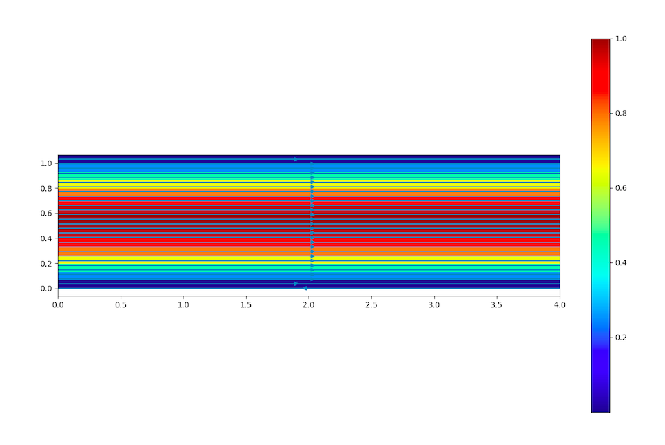
For further information go to the periodic Poiseuille flow documentation
Script for Poiseuille periodic flow:
    """Example on how to solve a Poiseuille problem  with the navier stokes solver"""

    import numpy as np
    import matplotlib.pyplot as plt
    from barbatruc.fluid_domain import DomainRectFluid
    from barbatruc.fd_ns_2d import NS_fd_2D_explicit
    #from barbatruc.lattice import Lattice

    __all__ = ["cfd_poiseuille"]


    # pylint: disable=duplicate-code
    def cfd_poiseuille(nsave):
        """Startup computation
        solve a poiseuille problem
        """

        width = 1.
        length = width*4
        dimx=length
        vel = 1.0
        t_end = 10.*length/vel
        nu_ = 0.01
        ncell = 15
        d_x = width/ncell
        dimy=width+d_x
        delta_x=width/ncell
        rho=1.12
        dom = DomainRectFluid(
            dimx=dimx,
            dimy=dimy,
            delta_x=delta_x,
            nu_=nu_,
            rho=rho)

        dom.switch_bc_ymax_wall_noslip()
        dom.switch_bc_ymin_wall_noslip()
        dom.fields["vel_u"] += vel
        dom.set_source_terms({
            "force_x": 8. * nu_ / width**2. * np.ones(dom.shape) * vel,
            "force_y": np.zeros(dom.shape),
            "scal": np.zeros(dom.shape)
        })

        print(dom)

        time = 0.0
        time_step = t_end/nsave

        #solver = Lattice(dom, max_vel=3*vel)
        solver = NS_fd_2D_explicit(dom, max_vel=1.8)
        for i in range(nsave):
            time += time_step
            solver.iteration(time, time_step)
            print("\n\n===============================")
            print(f"\n  Iteration {i+1}/{nsave}, Time :, {time}s")
            print(f"  Reynolds : {dom.reynolds(width)}")
            print(dom.fields_stats())
            dom.dump_paraview(time=time)
            dom.dump_global(time=time)

        y = np.linspace(0,1.07,num=1000)
        u=np.zeros(len(y))
        u_bulk=0.66
        Umax=(3/2)*u_bulk

        for i in range(len(y)):
            u[i]=Umax*4*(y[i]/dimy)*(1-(y[i]/dimy))
        plt.plot(y,u,color="red",marker="", label= 'theoretical curve')

        dom.show_profile_y()
        solver.plot_monitor()
        dom.show_fields()
        dom.show_flow()
        dom.show_debit_over_x()

        print('Normal end of execution.')


    if __name__ == "__main__":
        cfd_poiseuille(10)
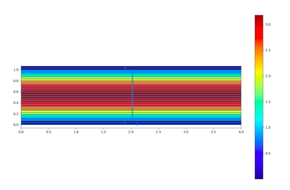
Second case:
This a Poiseuille flow with an input velocity and Re = 300
For further information go to the Poiseuille jupyter notebook. You will need to ask access to Nitrox to be able to follow the previous link.
It must give the following image. But be aware that the jupyter notebook is under construction and might not display the images because of a version upgrade.
Cavity
A lid-driven cavity simulation at Re = 300 will look like:
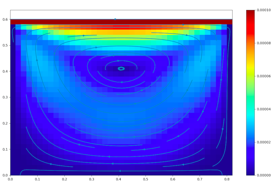
For further information go to the cavity documentation
Cylinder
The goal is to simulate Von-Karman street with a vortex-shedding frequency.
At Re = 100, we have a cylinder in cross flow:
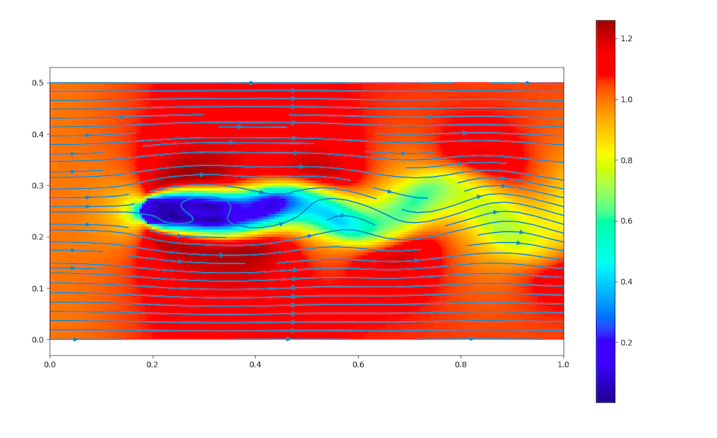
For further information go to the cylinder documentation