
The solutBound file manages the boundaries of the domain for AVBP. PyAVBP provides many ways to create or edit a solutbound.
Create any Solutbound from scratch
There is a crude helper function in pyavbp called gensolutbound().
It generates AVBP solutBound.h5 files without any check using a blueprint.
Better start with an example:
from pyavbp.io.mesh_utils import get_patch_size
from pyavbp.io.gensolutbound import gensolutbound

mesh_file = '../../Documents/MESH_C3SM/TRAPVTX/trappedvtx_perio.mesh.h5'
patch_sizes = get_patch_size(mesh_file)
bnd_targets =  [
    {
        "fields": {
            "RhoUn": {
                "value": 2.,
            },
            "Urms": {
                "value": 100.,
            },
            "mixture": {
                "value": [ 0.75, 0.25],
            },
        },
        "name" : "Inlet",
    },
    {
        "name" : "Outlet",
        "fields": {
            "Pressure": {
                "value": 101325.,
            },
        },
    },
]
mixture_species = ["O2", "N2"]
gensolutbound(patch_sizes, bnd_targets, mixture_species, "raw_solutbound.h5")
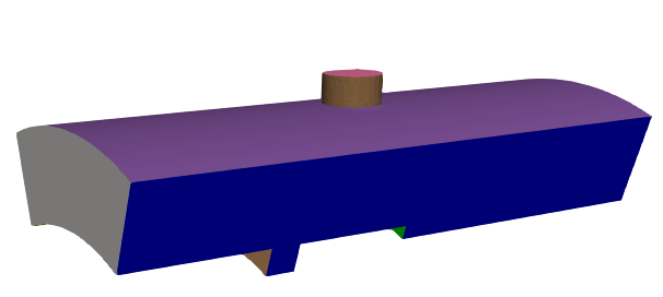
This small script creates a solutBound for the mesh trappedvtx_perio. Showing the data inside, we get:
>h5cross stats raw_solutbound.h5
+----------------------------+----------+----------+----------+--------+----------+
| Dataset                    |   min    |   mean   |   max    | st dev |  median  |
+----------------------------+----------+----------+----------+--------+----------+
| /Patch_001-Inlet/N2        |   0.25   |   0.25   |   0.25   |  0.0   |   0.25   |
| /Patch_001-Inlet/O2        |   0.75   |   0.75   |   0.75   |  0.0   |   0.75   |
| /Patch_001-Inlet/RhoUn     |   2.0    |   2.0    |   2.0    |  0.0   |   2.0    |
| /Patch_001-Inlet/Urms      |  100.0   |  100.0   |  100.0   |  0.0   |  100.0   |
| /Patch_002-Outlet/Pressure | 101325.0 | 101325.0 | 101325.0 |  0.0   | 101325.0 |
+----------------------------+----------+----------+----------+--------+----------+
Custom fields
However you can generate any kind of custom field, as long a you provide a numpy array of the correct shape. In this case, the inlet patch is defined by 417 vertices. Here we replace replace the value 2. of RhoUn by 2.*np.random.rand(417) -1.:
import numpy as np
(...)
bnd_targets =  [
    {
        "fields": {
            "RhoUn": {
                "value": 2.*np.random.rand(417) -1.,
            },
(...)
We get the same solutBound with a random field:
+----------------------------+-------------+-------------+------------+------------+-------------+
| Dataset                    |     min     |     mean    |    max     |   st dev   |    median   |
+----------------------------+-------------+-------------+------------+------------+-------------+
| /Patch_001-Inlet/N2        |     0.25    |     0.25    |    0.25    |    0.0     |     0.25    |
| /Patch_001-Inlet/O2        |     0.75    |     0.75    |    0.75    |    0.0     |     0.75    |
| /Patch_001-Inlet/RhoUn     | -0.99816073 | -0.01738461 | 0.98975535 | 0.57305945 | -0.02638937 |
| /Patch_001-Inlet/Urms      |    100.0    |    100.0    |   100.0    |    0.0     |    100.0    |
| /Patch_002-Outlet/Pressure |   101325.0  |   101325.0  |  101325.0  |    0.0     |   101325.0  |
+----------------------------+-------------+-------------+------------+------------+-------------+
So fields can be either a single scalar or a numpy array of the correct shape.
What if I mess up ?
If you mess up the shape, you will get the following error:
Traceback (most recent call last):
  File "/Users/dauptain/PYAVBP/GENPROFILE/trial_genprofile.py", line 94, in <module>
    gensolutbound(patch_sizes, bnd_targets, mixture_species, "raw_solutbound.h5")
  File "/Users/dauptain/GITLAB/pyavbp/src/pyavbp/io/gensolutbound.py", line 131, in gensolutbound
    boundary_target[bnd_p["name"]] = _create_boundary_data(
  File "/Users/dauptain/GITLAB/pyavbp/src/pyavbp/io/gensolutbound.py", line 91, in _create_boundary_data
    out[field] = scalar_array * bnd_fields[field]["value"]
ValueError: operands could not be broadcast together with shapes (417,) (418,)
If you provide a pathname not present in the mesh, you will get the following error:
Traceback (most recent call last):
  File "/Users/dauptain/PYAVBP/GENPROFILE/trial_genprofile.py", line 94, in <module>
    gensolutbound(patch_sizes, bnd_targets, mixture_species, "raw_solutbound.h5")
  File "/Users/dauptain/GITLAB/pyavbp/src/pyavbp/io/gensolutbound.py", line 133, in gensolutbound
    patch_data[bnd_p["name"]],
KeyError: 'InletXXX'
Takeaway
In a nutshell this gensolutbound() is only writing down to the disc what is in the blueprint bnd_target. All complex treatments (makeinject, genprofile, patchmapper) must be done before, in a non-AVBP, pure Numpy context.
Edit an existing solutBound
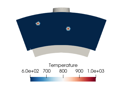
Add a hot spot
Here we want to add a hot spot at the inlet of the domain. We will directly edit the h5 file. There are plenty of Python packages to edit HDF files, some of them are described in this post. We choose to use h5py and hdfdict.
import h5py
import hdfdict
from pyavbp.io.h5_to_xmf_solutbound import write_xmf
We use with instructions to make sure the files are closed at the end of the script.
h5py is used to read the original file while hdfdict is used to transform the file into a dict and to render it easier to edit.
We also use PyAVBP’s write_xmf function.
with h5py.File('./oms_combu.solutbound.h5','r') as fin:
    solutbound_dict=hdfdict.load(fin)
    field=solutbound_dict['Patch_001-Inlet']['Temperature']
    solutbound_dict['Patch_001-Inlet']['Temperature'][100]=1000
    solutbound_dict['Patch_001-Inlet']['Temperature'][250]=1000
    with h5py.File('new_solutbound.h5','w') as fout:
        hdfdict.dump(solutbound_dict,fout)
write_xmf(meshfile, 'new_solutbound.h5', 'new_solutbound.xmf')
Apply a profile based on coordinates
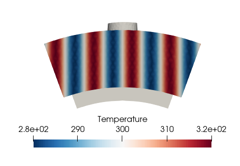
In this part, we will change a patch property according to the coordinates. For example, we want to apply a constant sinus-shaped temperature at the inlet.
# Some imports
We start importing the same packages as before plus a package to get mesh information and numpy:
import h5py
from h5cross import hdfdict
from pyavbp.io.mesh_utils import load_mesh_bnd,get_mesh_bulk
from pyavbp.io.h5_to_xmf_solutbound import write_xmf
import numpy as np
# Mesh manipulations
We use mesh_utils to get the coordinates of the points at the inlet patch:
solutbound_file = "./oms_combu.solutbound.h5"
meshfile = "../../COMMON/oms_combu.mesh.h5"
mesh = get_mesh_bulk(meshfile)
coord = load_mesh_bnd(meshfile)['Inlet']['xyz']
# Dict instantiation
Then, we use h5py to read the current solutbound and put it in a dict with hdfdict.
with h5py.File(solutbound_file,'r') as fin:
    datadict = hdfdict.load(fin)
We create a new array with the temperatures we want:
    new_temp = 300 + 20 * np.sin(coord[:,2]*50*2*np.pi)
    datadict['Patch_001-Inlet']['Temperature'] = new_temp
# Dumping the solution
We conclude by writing the new values in the dict and writing a new solutbound file:
    with h5py.File('new_solutbound.h5','w') as fout:
        hdfdict.dump(datadict,fout)
    write_xmf(meshfile, 'new_solutbound.h5', 'new_solutbound.xmf')
Apply a profile created with patchmapper
Disclaimer: This option is available only for patches with x constant profiles
Patchmapper is a tool that applies a profile defined as a numpy.array to an axisymmetric patch. You have to give it a dict with all the profiles you want to change and a reference array with key name ['rR'] along the height to make the interpolation. Make sure the lengths of the arrays in the dict are all the same, but not necessarily the same as the number of nodes in the patch.
# Some importations
We import the same packages as before for handling the HDF files, plus the package containing patchmapper and a package for mesh manipulation:
import h5py
import hdfdict
from pyavbp.tools import patchmapper as pm
from pyavbp.io.mesh_utils import load_mesh_bnd
from pyavbp.io.h5_to_xmf_solutbound import write_xmf
mport numpy as np
# Mesh and solutbound handling
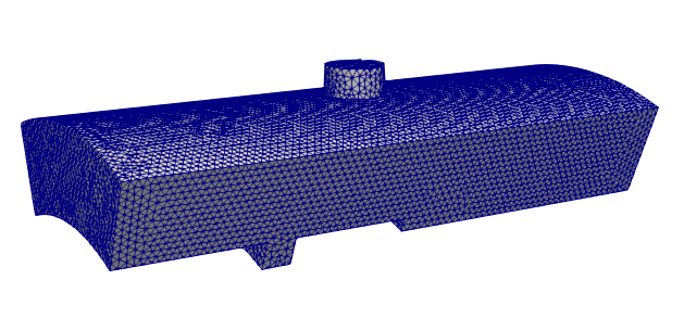
Now, we load the mesh and the solutbound files. We store the coordinates of the nodes for later:
solutbound_file = "./oms_combu.solutbound.h5"
meshfile = "../../COMMON/oms_combu.mesh.h5"
coord = load_mesh_bnd(meshfile)['Inlet']['xyz']
# Dict creation
We create the dict that we will use as an input of patchmapper. First, we calculate the radial coordinates of all the points of the mesh in order to find the extrema and to create the ‘rR’ entry of the dict for the interpolation made by patchmapper.
with h5py.File(solutbound_file,'r') as fin:
    datadict = hdfdict.load(fin)
    radial_points=2000
    radial_coord = np.hypot(coord[:,1],coord[:,2])
    profile_dict=dict()
    profile_dict['rR'] = np.linspace(np.min(radial_coord),
                                     np.max(radial_coord),
                                     radial_points)
Now, we can create all the entries we want in the dict. They have to be defined as vectors that will be interpolated on the mesh given the ‘rR’ vector. In this example, we create a temperature vector with a 1000K band and 600K everywhere else. The length of the hot band is one third of the total height located in the middle of the inlet patch:
    temp = 600 * np.ones(radial_points)
    temp[int(len(temp) / 3):int(len(temp) * 2 / 3)] = 1000
    profile_dict['Temperature'] = temp
# Patchmapper and dumping the solution
We call the patchmapper function with the right inputs. We change the initial dict with the new values. Then, we dump the new solutBound and the xmf file:
    new_fields_inlet = pm.apply_patchmapper_1d(profile_dict, coord)
    datadict['Patch_001-Inlet']['Temperature'] = new_fields_inlet['Temperature']
    with h5py.File('new_solutbound.h5','w') as fout:
        hdfdict.dump(datadict,fout)
    write_xmf(meshfile, 'new_solutbound.h5', 'new_solutbound.xmf')
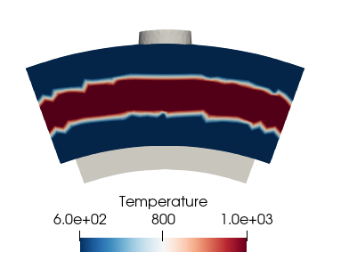
# The full code
import h5py
from h5cross import hdfdict
from pyavbp.tools import patchmapper as pm
from pyavbp.io.mesh_utils import load_mesh_bnd
from pyavbp.io.h5_to_xmf_solutbound import write_xmf

import numpy as np

#Mesh and solutboud handling
solutbound_file = "./oms_combu.solutbound.h5"
meshfile = "../../COMMON/oms_combu.mesh.h5"
coord = load_mesh_bnd(meshfile)['Inlet']['xyz']

#Reading the initial solutbound and initializing the output dict
with h5py.File(solutbound_file,'r') as fin:
    datadict = hdfdict.load(fin)
    radial_points=2000
    radial_coord = np.hypot(coord[:,1],coord[:,2])
    profile_dict=dict()
    profile_dict['rR'] = np.linspace(np.min(radial_coord),
                                     np.max(radial_coord),
                                     radial_points)

    #Creating temperature vector and applying patchmapper
    temp = 600 * np.ones(radial_points)
    temp[int(len(temp) / 3):int(len(temp) * 2 / 3)] = 1000
    profile_dict['Temperature'] = temp
    new_fields_inlet = pm.apply_patchmapper_1d(profile_dict, coord)
    datadict['Patch_001-Inlet']['Temperature'] = new_fields_inlet['Temperature']

    #Writing the new values in a new file
    with h5py.File('new_solutbound.h5','w') as fout:
        hdfdict.dump(datadict,fout)
    write_xmf(meshfile, 'new_solutbound.h5', 'new_solutbound.xmf')
Generalization with a CSV data to map on a patch
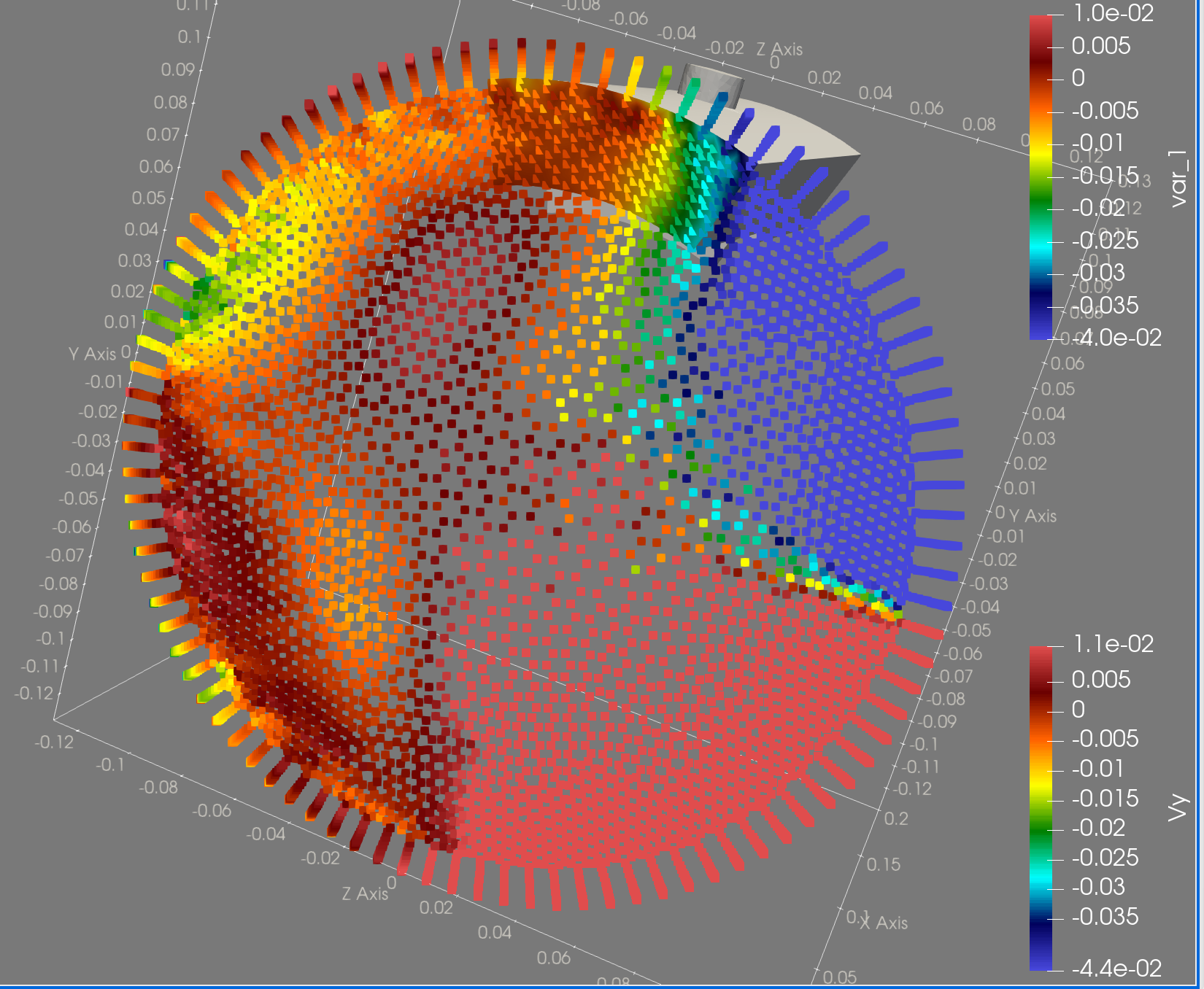
Here is a more advanced example where the origin data is not a profile but a point cloud provided in a CSV file. Copy and paste what you need…
import numpy as np
import matplotlib.pyplot as plt
import h5py
from h5cross import hdfdict
from pyavbp.io.mesh_utils import load_mesh_bnd
from pyavbp.io.h5_to_xmf_solutbound import write_xmf
from cloud2cloud import cloud2cloud
from arnica.utils.vector_actions import rotate_vect_around_axis
from arnica.utils.nparray2xmf import NpArray2Xmf

SIZE = 1000


def gen_fake_data():
    """Generate fake data if you do not have a CSV file for your tests"""
    rads = np.random.random(size=SIZE) * 0.1
    thetas = np.random.random(size=SIZE) * 2 * np.pi
    x = rads * np.cos(thetas)
    y = rads * np.sin(thetas)
    plt.scatter(x, y, c=y)
    plt.show()
    sce_coords = np.stack([x, y, 0 * x], axis=1)
    sce_data = np.stack([r, y], axis=1)
    return sce_coords, sce_data


def load_csv_file(filename):
    """Reading a csv file with only values

    We assume here thar the 3 first columns are X, Y and Z"""
    # Open and read the CSV file
    data = np.loadtxt(filename, delimiter=",")
    sce_coords = data[:, :3]
    # rotation de 90 degres autour de Y
    sce_coords = rotate_vect_around_axis(sce_coords, ([0, 1, 0], 90.0))
    # scaling pto fit on  trapped vortex mesh geometry

    sce_coords[:, 0] = sce_coords[:, 0] - sce_coords[:, 0].mean()
    sce_coords[:, 1] = sce_coords[:, 1] - sce_coords[:, 1].mean()
    sce_coords[:, 1] = sce_coords[:, 1] / sce_coords[:, 1].max() * 0.13
    sce_coords[:, 2] = sce_coords[:, 2] - sce_coords[:, 2].mean()
    sce_coords[:, 2] = sce_coords[:, 2] / sce_coords[:, 2].max() * 0.13

    sce_data = data[:, 3:]

    # plt.scatter(sce_coords[:,1],sce_coords[:,2],c=sce_data[:,-1])
    # plt.show()

    return sce_coords, sce_data


def projection():
    """Example of a solutbound where we change some fields and add other fields"""
    # Read source data
    sce_coords, sce_data = load_csv_file(csv_file)
    # A way to dump the data before interpolation
    dout = NpArray2Xmf("data.h5")
    dout.create_grid(sce_coords[:, 0], sce_coords[:, 1], sce_coords[:, 2])
    for i in range(6):
        dout.add_field(sce_data[:, i], "var_" + str(i))
    dout.dump()

    # load mesh data
    solutbound_file = "./oms_combu.solutbound.h5"
    meshfile = "./trappedvtx_perio.mesh.h5"
    csv_file = "FRONT_order.csv"
    coord = load_mesh_bnd(meshfile)["Inlet"]["xyz"]

    # projection
    projection = cloud2cloud(sce_coords, sce_data, coord, stencil=4)

    # editing the HDF5 file
    with h5py.File(solutbound_file, "r") as fin:
        datadict = hdfdict.load(fin)

        datadict["Patch_001-Inlet"]["var_0"] = projection[:, 0]
        datadict["Patch_001-Inlet"]["var_1"] = projection[:, 1]
        datadict["Patch_001-Inlet"]["var_2"] = projection[:, 2]
        datadict["Patch_001-Inlet"]["Pression"] = projection[:, 3]
        datadict["Patch_001-Inlet"]["Temperature"] = projection[:, 4]
        datadict["Patch_001-Inlet"]["var_4"] = projection[:, 5]

        # Writing the new values in a new file
        with h5py.File("new_solutbound.h5", "w") as fout:
            hdfdict.dump(datadict, fout)
        write_xmf(meshfile, "new_solutbound.h5", "new_solutbound.xmf")


projection()