AVBP’s temp files
AVBP dumps automatically several files while running a simulation. These files are stored in the TEMPORAL folder and give precious information to monitor the run.
The same TEMPORAL folder contains the probes specified in the probe_file (usually record.dat).
You can display some information of these files with PyAVBP’s command line entries pyavbp bin-read, pyavbp bin-head and pyavbp bin-plot.
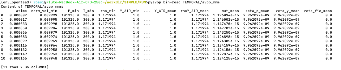
But if you want to get these values and make a treatment on them, you might be interested in using PyAVBP’s readbin tool.
Readbin
Get the data
Getting the data is very easy. All you have to do is to import PyAVBP’s readbin and to call it with the path to the file you want to explore:
from pyavbp.io import readbin

data = readbin('TEMPORAL/avbp_mmm')
The data you get is of type BinData. It is kind of a dict so it is readable by Pandas, a very useful package for data analysis.
Creating a DataFrame
Pandas main functionnalities are built on an object called a DataFrame. Its interest is that you can handle your data like a two entries table where each column is a variable and each row is a time record.
import pandas as pd

pd_data = pd.DataFrame(data)
| atime | norm_vel_min | P_min | T_min | … | |
|---|---|---|---|---|---|
| 0 | 5.708319e-07 | 2.876862e-18 | 101324.962105 | 299.999968 | … |
| 1 | 2.853341e-05 | 1.442791e-16 | 101323.068941 | 299.998368 | … |
| … | … | … | … | … | … |
Small trick: The
describemethod displays interesting information on your dataset like the mean, standard deviation, quantiles…
pd_data.describe()
              atime  norm_vel_min          P_min       T_min  ...
count  3.000000e+00  3.000000e+00       3.000000    3.000000  ...
mean   2.871816e-05  3.284584e-16  101323.078464  299.998376  ...
std    2.824015e-05  4.470914e-16       1.878898    0.001588  ...
min    5.708319e-07  2.876862e-18  101321.204346  299.996793  ...
25%    1.455212e-05  7.357797e-17  101322.136643  299.997580  ...
50%    2.853341e-05  1.442791e-16  101323.068941  299.998368  ...
75%    4.279182e-05  4.912491e-16  101324.015523  299.999168  ...
max    5.705022e-05  8.382191e-16  101324.962105  299.999968  ...
Little preview of Satis
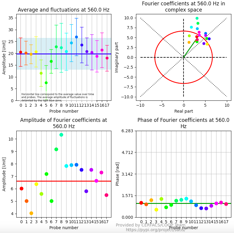
Satis (Spectral Analysis of TIme Signals) is a COOP package you may find interesting to use to make spectral analysis on your temporal records. It is a package which can calculate the Power Spectral Density (PSD) of your signal(s) and provides tools about temporal analysis.
Here is an example of how to create a file to use Satis:
p_min = data['P_min']
with open('my_dataset.dat', 'w') as fout:
    for idx, time in enumerate(data['atime']):
        fout.write(f'{time} {p_min[idx]}\n')
And here you have an example of the kind of plots you can display:
Data analysis
Pandas DataFrame structure is specially suited to make data analysis. You can now dump your data in a csv file with pd_data.to_csv('myFile.csv', sep = '\t') and open it in a Jupyter Notebook. A tutorial on how to make data analysis on a Jupyter Notebook with Pandas can be found here.