Reading time: 17 min

A supercomputer is designed to perform high-speed calculations much faster than a regular computer. The insights generated help experts to answer advanced questions : Does this theoretical model agree with observations? Is this cooling device strong enough to protect the engine? Naturally, the operating cost of these very expensive facilities is monitored closely.
Computational waste is becoming a significant problem in the world of supercomputing. It refers to the inefficient use of computing resources, such as having a supercomputer sit idle for long periods or running jobs that ultimately produce no meaningful results. This waste might be negligible today, but as computing power increases, wasted ressources increase too. For example, the exascale Aurora will consume 60MW of electricity. One percent of its production during one year at a cheap 10cts/KW.h price means 0.525 millions of US$, just for electricity. Oops!
In this blog post, we want to bring attention to the central role of supercomputer users in the mitigation of computational waste. In a nutshell, a lack of awareness is letting users run with wasteful behaviors. Therefore, after a brief recall of what running a supercomputer means, we will introduce new metrics for measuring computational waste, then we will describe the two main waste sources: understayers jobs and overstayer jobs. Finally we will show how we can engage users in this quest for better and cleaner workloads.
Maybe this was too technical from the get-go, so here is an other angle. Let’s express the problem from the point of view of an anthropomorphized job scheduler:
Greetings, it’s Sheldon, the all-knowing job scheduler for a supercomputer. My job is to manage the queue of jobs submitted for computation. It’s a tough gig, especially when users can’t file a job request properly. Last year, a whopping 40% of my precious production jobs crashed before even getting started! Can you believe it? Even if they don’t stick around, they still managed to make me delay my production lines for them, all for nothing. And that’s not all. Another 40% finished before the halfway mark when they could have easily been squeezed into empty slots. These understayers are jamming up my waiting line every five minutes.
And don’t get me started on those pesky jobs that run until the machine kicks them out, wasting days of computing time each year. Do these overstayers know that the last bit of computation cannot be saved? Apparently not. But who cares, right? When people move on to exascale computers, their blunders will bring fire and fury. Until then, I’ll just keep rolling my eyes and repeating, “I’m not paid enough for this.”
Ok, Sheldon is overreacting, and supercomputing systems work just fine. The point is they could do much better with a bit of training, and we will outline some strategies for reducing computational waste…
Running on a supercomputer, a primer
This section is an introduction to the mindset of a supercomputer runner. As an analogy, we will think of a run as a large number of containers that must be shipped across the sea.

The simulation volume
We name here a simulation a digital model of the problem considered running for some time on the machine. For example, the air volume surrounding a wing is represented by \(n_{pts}\) sample points defining a grid that tiles the geometry. Each sample point holds several \(n_{var}\) variables : speed, temperature, density, gaz composition, etc… Their product measures the degrees of freedom: \(dof = n_{pts}*n_{var}\)
An iteration It is a cycle where all dof are updated. Each update involves several Floating Point OPeration (FLOP). Thus, the Volume of the computation , expressed in FLOP, is the number of iteration times the degrees of freedom:
\(Vol=\alpha*It.*dof\)
With \(\alpha\) the average number of FLOP per dof within one iteration.
In other words, the volume of the digital model is the volume of the cargo to ship.
Running the simulation
The user must request ressources for a while. Let’s say \(n_{cores}\) computational cores for a duration \(t_{lim}\). (read an analogy to understand supercomputers for a complete description of computational cores). In the cargo analogy, it is \(n\) container ships booked for \(t_{lim}\) monthes from the same shipping company.
Each node has a computing speed expressed in FLOP per second (FLOPs). The actual speed (\(c_{real}\)) for our simulation is the peak speed of the node (\(c_{peak}\)) times the software efficiency (\(eta\)) for this case and resource:
\(c_{real} = c_{peak}*{\eta}\)
The real job duration is therefore, for \(n\) nodes.:
\(t_{job} = Size/(n_{cores}*c_{real}) = (\alpha/\eta) * (It. * dof) /(n_{cores}*c_{peak})\)
This formula gives you the baseline parameters. The separate values of \(\alpha\) (FLOP per DOF) and \(\eta\) (% of peak perf.) are not trivial to evaluate. However, once one job is done, the ratio \((\alpha/\eta)\) is known. Obviously, one request the ressources for a duration \(t_{lim}\) a bit longer than \(t_{job}\). Back to the cargo analogy, the user booked 8 ships (\(n_{cores}\)) for maximum 6 months (\(t_{lim}\)). They processed the whole cargo in 5 monthes and one week (\(t_{job}\)).
How users can waste ressources?
The scheduler is ordering all the requests to maximize the resources and the user satisfaction. In our cargo analogy, scheduling means planning the missions of all ships in the company. Groups of ships are dedicated to one workload for some weeks. Some ships are more suited than other for a mission. Now see what happen when things go wrong. Each job need to ready all ressources at starting time.
If the job crashes , all ressources are freed (no-stayers). Now, imagine the gathering of a fleet of empty container ships, disbanded once they are together. All this idle ships are ressources wasted for the company.
When most jobs are much shorter than planned (understayers), the production schedule will appear more loaded than reality, and changes constantly. In other words, users are jamming themselves their vision. In addition, some jobs can fit in the idle spots of the workload if they are short enough.
Finally, a job longer than the requested time (overstayer) is abandoned without saving anything. This is the same as a ship dumping the cargo in the sea before moving to the next mission. This last mission is lost for the current customer (part of cargo lost), the next customer (delayed start) and the company (fuel burned).
What about the queues?
The “queues” are predefined job families. The most common are: * The debug queue, often less than 30 minutes on one single node. * The production queue, usually 6 hours nearly 20% of the resources. * The long queues, 24 or 48 hours up to 50% of the machine.
See an example from Ohio Supercomputer Center’s “Oakley” queues . There is often a table recording the available queue looking like:
| Name | Max walltime | max job size | notes |
|---|---|---|---|
| debug | 0.5 hours | 1 node | two nodes reserved |
| prod | 6 hours | 32 nodes | |
| long | 24 hours | 64 nodes | |
| weekend | 48 hours | 128 nodes | start on Sat. & Sun. |
Queues vary in terms of restricted access, reserved nodes for constant availability, and can redirect to different kinds of nodes from the same machine. Some systems simply use the job definition (resources, duration) to identify the queue. On other systems, one states the queue, then overrides some parameters (e.g. reducing the duration).
What about the partitions?
The word “partition” can have different meanings. Initially, it refers to a subset of the resources. For example, the “Skylake” partition and the “IceLake” partition can be two families of processors installed on a machine. The “debug partition” can be two nodes exclusively dedicated to debugging, accessible only by the queue “debug”.
Because of the close relation between a queue and a partition, the terms are often mixed. There are actually supercomputers where each partition is accessible by a single queue of the same name. If you are not an administrator, maybe simply avoid using the term “Partition”.
One year worth of jobs
Let’s recapitulate a job request :
- the number of nodes \(n_{cores}\) (the nuber of ships)
- the duration of the job \(t_{lim}\) [s], a.k.a. Time Limit, Wall Time, Requested Time, etc…
The following figure shows all jobs of 2022 on our small supercomputer “Kraken”, our petaflop internal cluster.
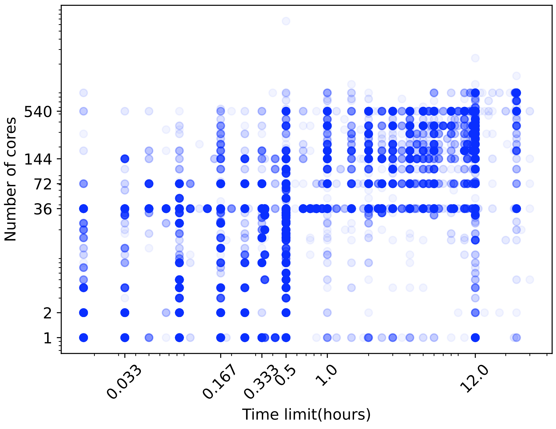
All the jobs of year 2022 submitted on Kraken, our petaflop internal cluster. The five most frequent time limits set are 5min, 10min, 20min, 30min, 1hours and 12hours.
This shows mostly small jobs -few resources for short duration- used for debugging, and large jobs -large resources for long duration-.
| short duration | long duration | |
|---|---|---|
| large resources | large scale test | production |
| small resources | nominal test | aborted production |
The cumulated production of a cluster is often over 90% of the maximum production. When demand is too high, users judge that now is not the time to run. The user experience of the cluster is very often reduced to this waiting time:
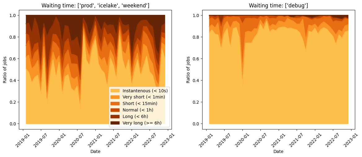
Monthly share of job waiting times for our cluster Kraken on the production queues (left) and debug queues (right).
In this figure, we show the repartition of waiting times observed by users along fours years. The wait on production runs (left) is much higher than the debug runs (right). However, a small share of debug jobs are very slow to start, often because during weekends, productions queues have top priority. The organization of the waiting line seems to be tricky after all.
The waiting line
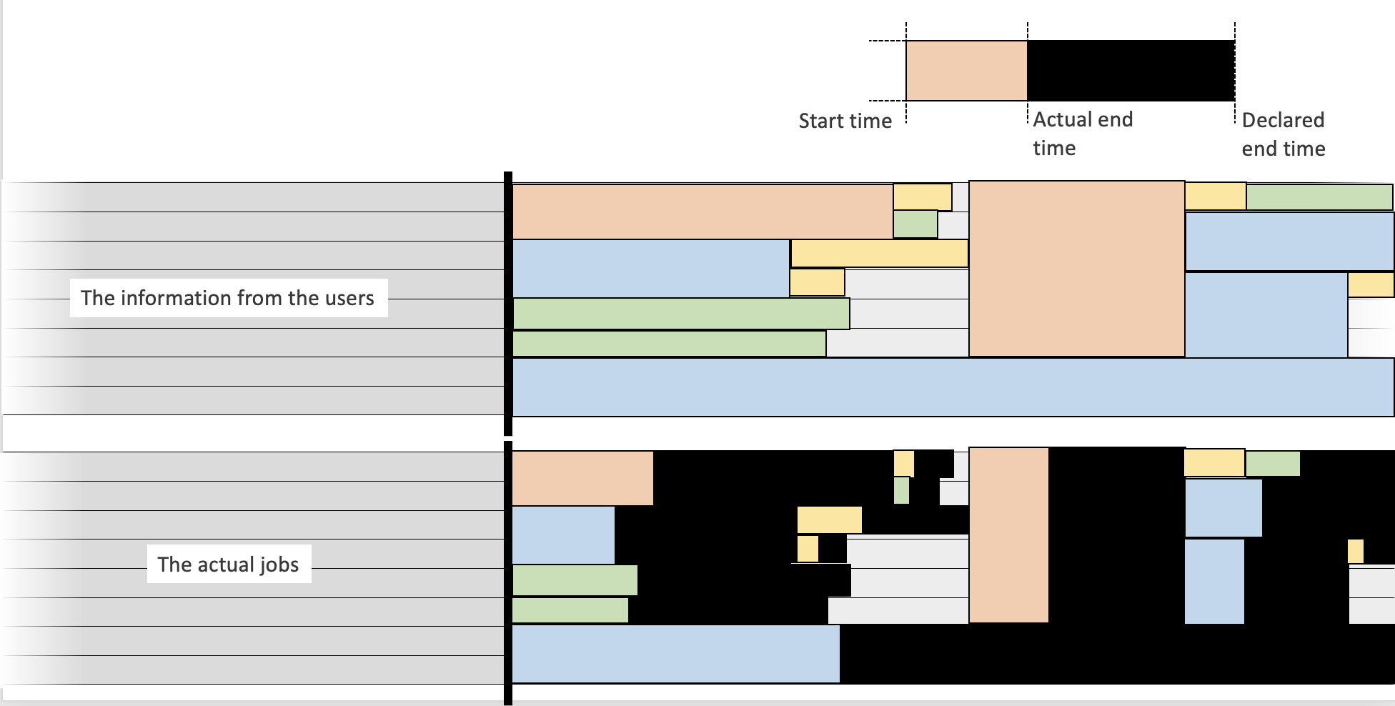
The waiting line for an HPC cluster is like a conveyor belt. Jobs are represented as boxes that move towards the processing machine. The width of the conveyor belt corresponds to the total number of available resources, while the length of each box corresponds to the job’s duration.
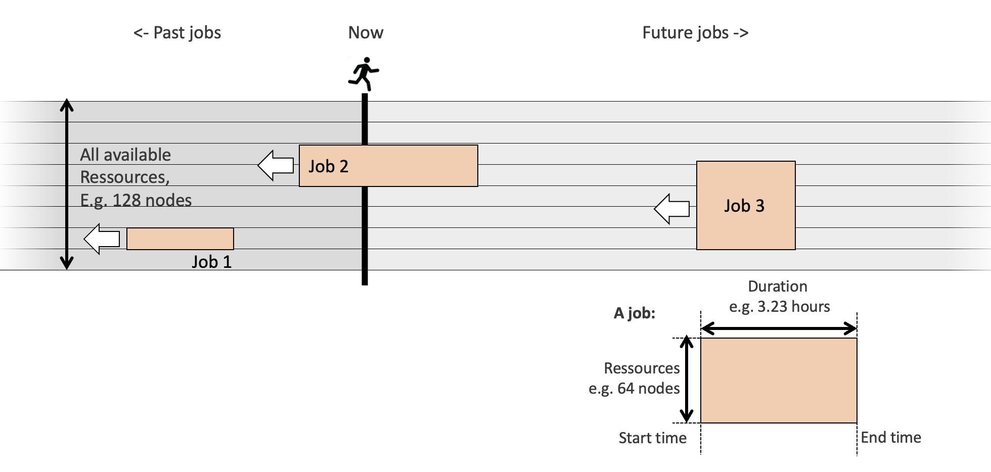
The waiting line, or queue, is like a conveyor belt. Each job is a box of with \(n\) and length \(t_{lim}\). The belt advances the box toward the processing line.
The total number of resources sets the width of the conveyor belt. For example, a job using all the resources is a box that would span the full width of the belt. In the other direction, the length of the box is the duration. A 12 hour-job takes twice as long as a 6 hour-job.
The job scheduler
The job scheduler places each box on the conveyor belt as close to the processing line as possible, following a “First In First Out” (FIFO) rule. If two jobs arrive simultaneously, the scheduler gives priority to the user who used fewer resources recently, according to the Fair Share policy.
The jobs, tightly tiled to optimize the use of the ressources.
If two jobs similar in size arrive at the same time, the scheduler will look at the users records, and promote the one who used the least resources recently. Rules to determine priority vary around the concept of “big runners have lower priority”. This is named Fair Share (Read more on the Slurm Scheduler HomePage).
The way you send a request vary from a scheduler to another, but the content fit in the same form. As a proof, play with NERSC’s unified form which translates the same requests to four different machines.
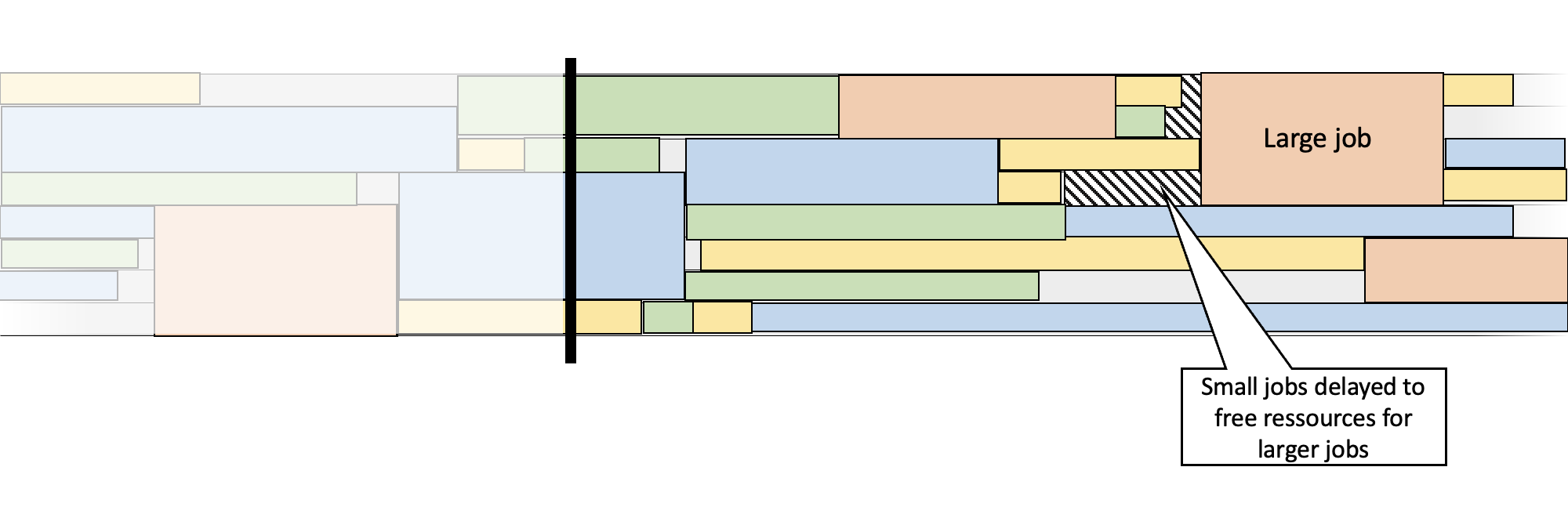
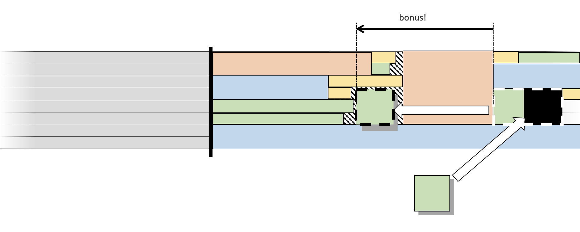
Large Jobs and Backfill
To accommodate larger jobs, the scheduler may set some resources idle, resulting in a loss of production. However, the Backfill process allows smaller jobs to fill gaps in the workload created by these idle resources. This helps to mitigate the impact of large jobs on overall productivity.
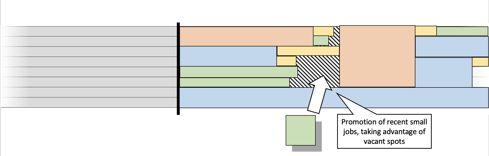
Backfilling. The green new job was not First In, but it can fill a spot, so it is promoted.
Showing the inacurracy of users requests
the accuracy is the actual run time \(t_{job}\) divided by the requested wall time \(t_{lim}\). Accuracy near 0 is for instant crashes (yellow) , near one for time-out jobs (dark brown). The figure shows that 80% of submitted jobs are largely overestimated, and 10% wait for being kicked out by the system.
Let’s see the figures on an actual workload from our internal clusters:
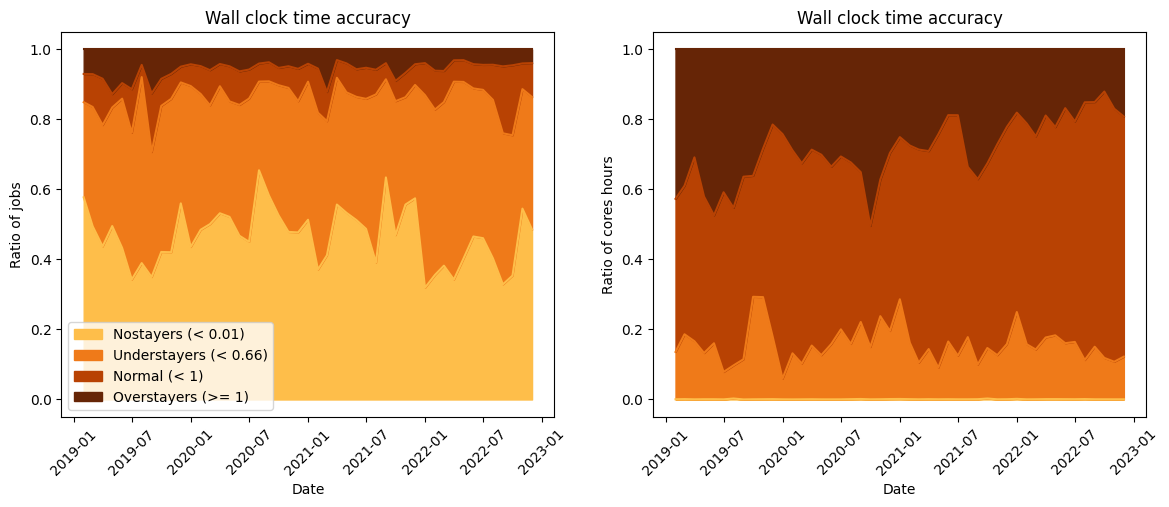
Share of jobs in terms of accuracy, on production partition, showed as the raw job number share (left) then as the consumed hours share (right)
The data exclude all jobs done on debugging ressources, and focuses only on production ressources (long and large jobs). This datavisualization highlights the three bad running habits of users:
Nostayer jobs (in yellow on the figure)
The “no-stayer” jobs are extreme understayers, less than 1% of the requested time. Even if they did not use a lot of resources, their spot was reserved in the workload.
Most of “no-stayers” are trivial issues : a permission problem or a wrong path cancels the job before any computation. In research, there are also quick crashes. Our digital models are often as instable as they are precise. Tuning the right parameters are done either with carefully selected tests, analyses and discussions, or many trials and errors. The latter is a very bad temptation of course: The spots of all No-stayer jobs jobs are reserved nevertheless, accumulating small idle times in the global production
The “no-stayer” jobs impact is almost cancelled when users always prepare their run on “debug” queues. The idle ressources are smaller, and the waiting time is usually below the minute.
Understayer jobs (in bright orange on the figure)
An “understayer” job is significantly shorter than the requested time - let’s say a duration lower than 66% of the requested time. The computation being successful, most users never realize it was an understayer job.
Understaying, if done one a large scale, feed the scheduler with essentially wrong information.
If a job duration is correctly estimated, the backfill process puts the job earlier in the queue. The result delivery is done hours earlier, which is more effective than any performance optimization.
A user can gain a lot of time with better prediction of the time limit.
As there is no feedback saying “you could have got this result 8 hours earlier with a better duration estimation”, understayer jobs represent a large part of the workload. IBM Spectrum LSF is one of the major player of HPC schedulers. In the 2018 communication A Crystal Ball for HPC, they showcased a feature able to predict the proper time-limit to maximize resource.
Here, users can monitor their jobs with the sheduler command line and by reading the jobs logs . As logs are quite technical and extensive, a supervisor must help them to know where to look.
Overstayer jobs (in dark brown on the figure)
On the other side of the spectrum, some jobs run until being kicked out. It is a Time-out. Most HPC softwares use checkpoints, i.e. save enough data to restart for there. For a time-out, no data can be saved.
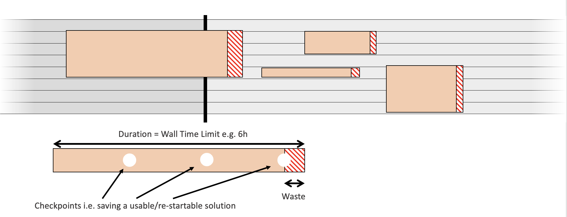
By overstaying, a user do some computation which cannot be saved. The ressource used could be freed for someone else.
If you sum the resources wasted by overstayer jobs, which are large production jobs for most of them, you get a substantial amount of pure waste. Assuming 5% of waste (20 checkpoints per job) for a year of overstayer jobs, this was a loss of nearly 3 days of production on our cluster.
Similarly, users can spot overstayers by reading their jobs logs. Morevover, If a mail is sent by the scheduler to the user, one can easily create a custom warning by filtering the mails.
What can be gained with a better user accuracy ?
If the no-stayers and understayers jobs are mitigated, the idle time of ressources will decrease. The overall production of the machine could increase by 5%. Runs moved to a debug queue or benefiting a backfill will deliver results hours earlier to the users. In addition, the schedule of job will be much more accurate. If overstayers jobs vanish, around 1% of the total production would become usable. Remember that, as the power of supercomputers increases, the cost of waste also increases. For example, if 1% of the yearly production of an exascale system is wasted, literally millions of USD are lost in pointless energy.
Engaging users in the quest for better workloads
Apparently, most users are not aware of the good habits.
We avoided writing yet another bullet list of good practices, because our users declared they rely more on mouth-to-ear tips from peers than re-reading training slides and online documentations.
Instead, we developed user-oriented datavisualization of the past workload, and the Top 5 best users was designed precisely to identify the people to follow. The process of ranking is the following:
- In a month, list all users who submitted jobs on the production queues (i.e. exclude all debugging jobs)
- Count the jobs submitted in production during the month
- Discard users that submitted less than 10 jobs this month
- Compute the job duration accuracy: job duration / time requested
- Sum jobs with accuracy < 0.01 (No stayers), < 0.66 (Understayers), > 0.99 (TimeOut) as Total Bad Jobs
- Compute the ratio 1-(Total Bad Jobs)/(Total jobs)
- Rank users…
In a nutshell, score is set to 1 for active users, and decrease each time a job duration is not fitting well the requested time. Finaly, we created the following figure to promote good users:
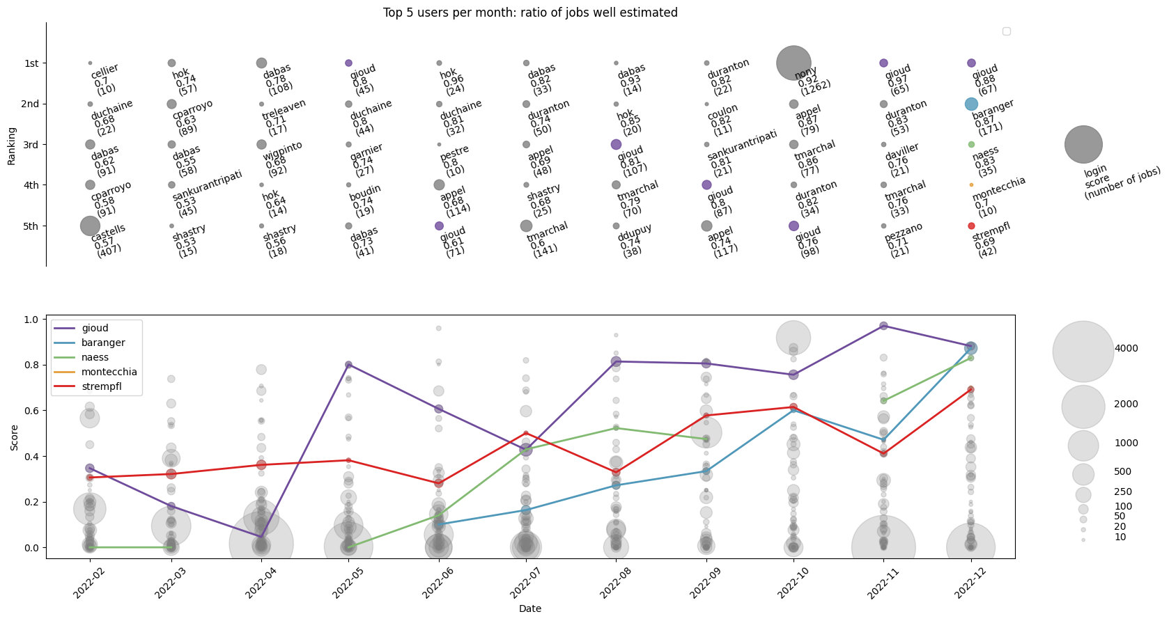
Example of a monthly top user ranking based on how accurate and successfulm the jobs were.
In this example, Gioud, Baranger and Naess are respectively the top 1,2,3 users of Dec. 2022 Their past scores is highlighted with colors, and all show a positive global trend with time. This illustrates how they learnt to reduce the waste with experience. Note that on october, Nony reached the first place with 92% of his 1200 jobs well shaped in one month. An in april and november, some users submitted 4000+ jobs per month with a score of almost zero…
Note that most global communication towards users is negative, e.g. “these are the 10 biggest consumers of last month”. This can trigger unofficial shaming, like “did you really needed that much ressources…, aren’t you just blindly chaining jobs, etc…”. We decided to do exactly the opposite, and first feedback are good.
Facing this datavisualization, our users saw that some people they know personally are quite good at shaping their jobs requests, and plan to ask them some tips. They also realized that top consumers list and best users list are not correlated. Finally, some pointed out that very bad performers (thousands of jobs with a quasi null score) were visible. They think that farming bad jobs becomes less tempting if you know you they can be spotted.
Takeaway : users have a central role in the workload optimization
Many supercomputer users are not aware of good practices for optimizing their simulations workload. Instead of relying on traditional training materials, users tend to prefer tips from their peers. Additionally, most communication towards users about their usage of the supercomputer tends to be negative, which can lead to unofficial shaming.
The traits of a better request to reduce computational waste are:
- Ask for a duration a bit longer than the time needed. Neither too long, nor too short.
- Do sanity checks (permissions, file path, etc…) on debug queues before the submission to avoid instant large crashes (nostayers)
- Keep away from the temptation of farming trial-and-error large jobs (nostayers)
- Keep watch on the jobs logs and the accounting reports.
With this in mind, users can increase the available resources, and largely impprove ther user experience.
To address this problem, a user-oriented data visualization was created that ranks the top five best users based on their job accuracy and success rate. This visualization promotes good users and identifies the people to follow for tips on optimizing their workload. The ranking system is based on a score that decreases each time a job duration is not fitting well the requested time. The data visualization also shows the progress of top users over time and how they learned to reduce waste through experience. By showcasing good performers and promoting positive feedback, the hope is to encourage more users to adopt good practices and reduce the temptation to farm bad jobs.