![]()
Disclaimer : This post is not finished and has NOT been fully reviewed. Feedback are welcome, but no arguments (yet) please!
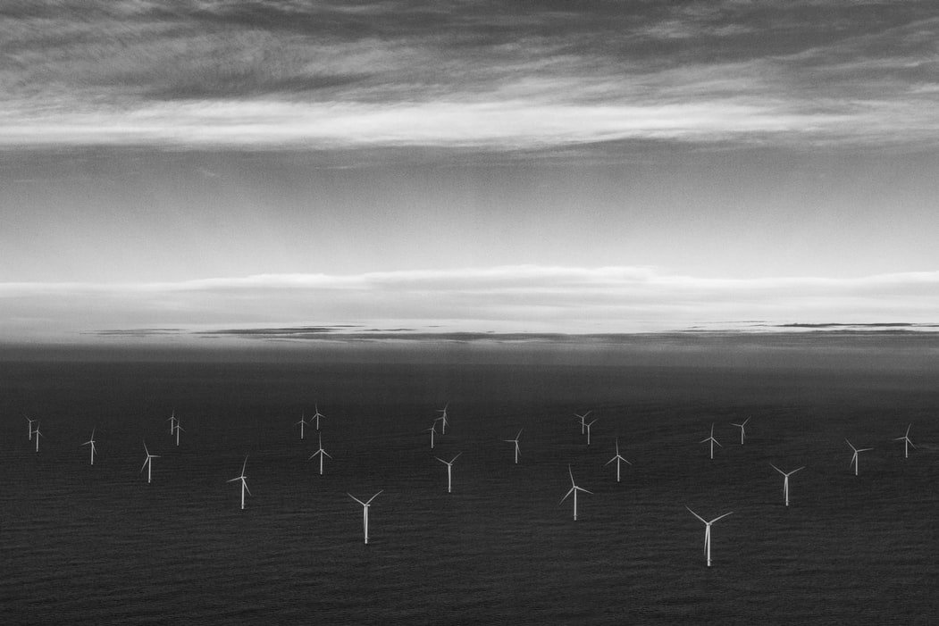
An offshore wind farm is a challenging fluid dynamics configuration. The atmospheric boundary layer is, in itself a very rich topic. Coupling wind turbines with this flow is even harder. Cerfacs will start a research activity soon on this. In the meantime, this post illustrates our tech-watch first experiences.
Introduction
The “WindFarm Challenge” aims at the step-by-step evaluation of different numerical approaches to simulate an off-shore wind farm. The reference publication used for the target flow here is Calaf et al., in Phys. Fluids 2010. As there is a large literature on the topic, start your bibliography with MeteoFrance Ph.D. Thesis of Q. Rodier (2017).
Currently we only tested a Finite Volume/ Finite Element code solving the Navier-Stokes equation, AVBP, and a Lattice Boltzmann Solver, WalBerla, on the first babysteps on the path towards a WindFarm simulation.
First we study a laminar test case, then try to extend to a turbulent case.
Flow characteristics
The fluid used to run the case shows the following characteristics :
!---------------------------------------------------------------------------------------------------------------------
! Non reactive mixture AIR.
!---------------------------------------------------------------------------------------------------------------------
  mixture_name = AIR
  transport = computed
  combustion_chemistry = no
  species_name = AIR
  species_Schmidt_number = 1.d0
  viscosity_law = sutherland
  mu_ref = 1.716d-5
  T_ref = 273.15d0
  viscosity_law_coeff = 110.6d0
  prandtl_number = 0.71d0
The numerical configuration is :
Geometry :
- Lx = 110000m
- Ly = 2000m
- Lz = 3100m
- delta_x = delta_y = delta_z = 100m
Boundary Conditions :
- en y = 0m : No_Slip
- en y = 1000m : Symmetry
- Periodic along X and Z
Initial conditions :
- P = 100000Pa
- T = 300K
- Speed = 0 m/s
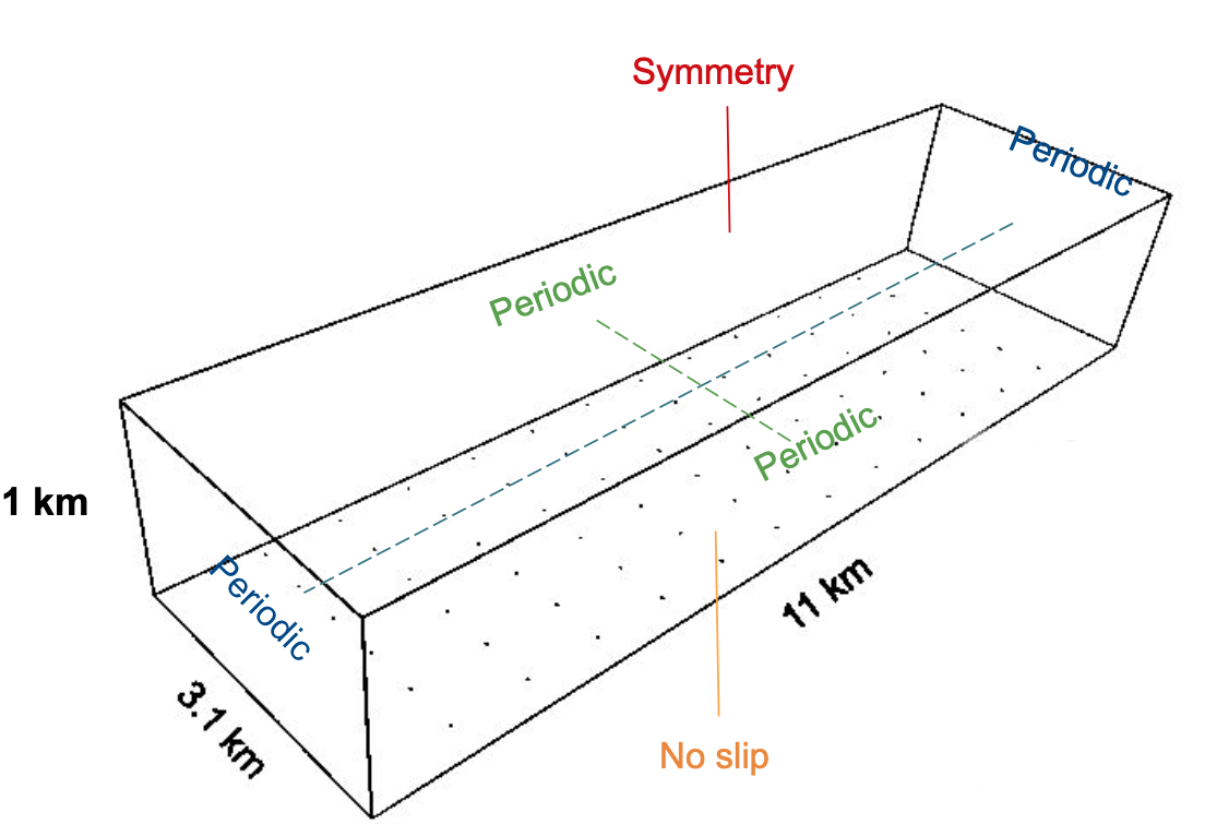
Finally, we’ll use a quad mesh (as this type of mesh is the most commonly used in LBM).
The Laminar Test case
To make the case laminar, we need a much more viscous fluid, nicknamed “air lourd”. We chose the parameters in order to get a speed of about 23m/s at the center of the channel (the velocity we’re supposed to get while running the turbulent test case : CF turbulent WFC AVBP). Note that heat capacity has been increased accordingly : with such a viscosity, the Joule effect heats up the fluid, and both temperature and Pressure would significantly rises during the simulation.
!---------------------------------------------------------------------------------------------------------------------
! Non reactive mixture AIR_LOURD.
!---------------------------------------------------------------------------------------------------------------------
  mixture_name = AIR_LOURD
  transport = computed
  combustion_chemistry = no
  species_name = AIR_LOURD
  species_Schmidt_number = 1.d0
  viscosity_law = sutherland
  mu_ref = 1.d+3
  T_ref = 273.15d0
  viscosity_law_coeff = 110.6d0
  prandtl_number = 0.71d0
In this laminar case, we don’t have any turbulence model, Forcing term along x : 0,05 kg/m2/s2.
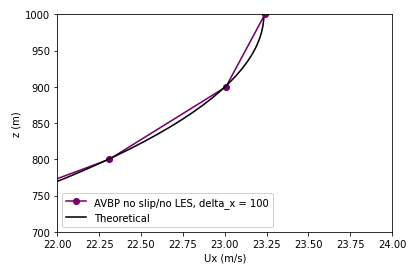
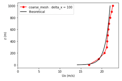
AVBP
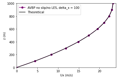
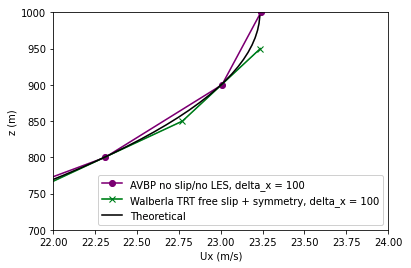
At the end of the simulation, we can get the following profiles that we compare with the theoretical curve. As we can notice on the previous picture, the calculation has converged.
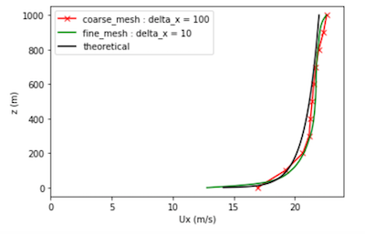
Now let’s run the same case on a fine mesh (delta_x = delta_y = delta_z = 10m) :
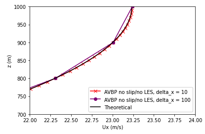
Here, we can notice that both curves are perfectly matching.
waLBerla
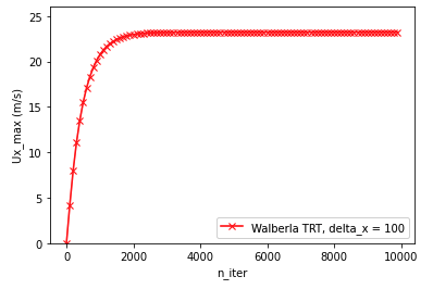
Now, let’s do the same work with waLBerla. For the collision operator, we use a two relaxation time model. For more information about LBM models, CF here. Concerning the initial conditions, we have speed = 0 m/s everywhere and we set a temperature of 300K (which isn’t going to change, the models used in waLBerla use the isothermal hypothesis).
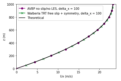
At the end of the simulation, we can get the following profiles that we compare with the theoretical and AVBP curves. As we can notice on the previous picture, the calculation has converged.
Now let’s run the same case on a fine mesh (delta_x = delta_y = delta_z = 10m) :
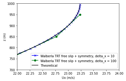
Here, we can notice that waLBerla perfectly matches AVBP and the theoretical curve.
The Turbulent Test case
In this turbulent case, we are using a Smagorinsky turbulence model. We set the value of the forcing term along x to 0,00024806 kg/m2/s2.
The Mesh size is increased by a Thousand (Delta X=10m). This is far insufficient for a proper Law of the Wall imposition (Y+ around 300000!!!), but physical modeling is not the point yet. This is just a numerical testbed for now.
The turbulent test case has already been implemented and commented on AVBP : turbulent WFC AVBP.
AVBP
Let’s now talk about the turbulent case model on AVBP. We need a wall Law in order to properly model turbulence at the wall :
!------------------------------------------------------
patch_name = Wall
boundary_condition = WALL_LAW_ADIAB
free_corner_min_angle = 60.0d+0
At the end of the simulation, we can get the following profiles that we compare with the theoretical curve. As we can notice on the previous picture, the calculation has converged.
Now let’s run the same case on a fine mesh (delta_x = delta_y = delta_z = 10m) :
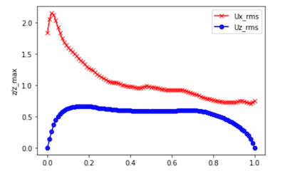
You’ll find below the velocity fluctuation profiles.
There is a lot more to do to improve the simulation from the physical point of view, the first being to move to a Y+ close to 200 at the wall. We can however take some performances out of this.
HPC performance on production capacity.
The HPC performance will be expressed here in terms of production capacity:
-
Solvers will run the same fluid configuration.
-
Solvers will be run on an equal amount of degrees of freedom, denoted as “Fine Mesh”.
-
Solvers will be run on an same computer and queue for the same duration, denoted as “production run”. For example, out first test is is the nominal production queue on the Cerfacs’s in-house Kraken cluster.
-
Solvers will use a fair-enough nominal version of their sources. For example, we shall not comment manually the lines of codes or change the equations usually solved.
This comparison is practical but unfair. Indeed, focusing only on the production capacity, it does not take into account the amount of supplementary modeling, nor the numerical precision.

This production capacity competition is similar to the Eco-marathon shell idea: with the same amount of fuel, how far can you go?
The classical Production CPU queue
The present resource here is :
12 hours on 15 nodes , a node being two Intel Xeon Gold 6140 processors, each featuring 18 cores Skylake processor at 2.3 Ghz. The maximum consumption allowed is therefore 6480 CPU hours.
| Code | Laminar | Turbulent |
|---|---|---|
| waLBerla | 46h | N/A |
| AVBP | 0.45h | 0.66h |
| AVBP-PGS | 0.45h | 2.64h |
Physical time simulated with one production run on Cerfacs cluster Kraken
We expect the waLBerla framework to show better performance, due to the code generation approach and the modeling “sobriety”. It is however unable to perform Wall-law cases for the moment, making it unable to comply to the turbulent case. On the other hand AVBP, with a non-isothermal, variable Cp, multi-species, compressible formulation, is largely “over-modeling” the case. Both codes are probably not at their maximum level of performance yet.
This numerical testcase is a first step on very coarse meshes, to get a qui time-to-solution. In real life, the meshes would be extremely heavier, which would eventually impact the performances. Take these figures with the utmost caution.
The “Kiss and cry” corner
Read these elements before filing any complaints:
-
Due to its blocking system, waLBerla could only use 30 cores on the 36 available per node, losing 20% of the bandwidth before the competition even started. waLBerla is also not featuring a law-of-the-wall turbulent boundary condition, disqualifying any attempt on the turbulent case for the moment.
-
AVBP is a compressible solver, a disadvantage for convection at low Mach numbers. The AVBP-PGS mode decreases artificially the sound speed, making the solver similar to an artificial compressibility code, the PGS allowing a x4 PGS boost (25m/s becomes Mach 0.3!). AVBP-PGS releases the constraint on the convective limit, but the laminar case is constrained by the diffusion limit. The PGS boost is therefore nullified.
Future work
We plan to extend this challenge to other current production queues, the most interesting being obviously GPU partitions, in the size and state available today. The post processing will also be extended to variance profiles and autocorrelations times and lengths.
If you think you can do better with AVBP or waLBerla, but also MESO-NH, JAGUAR, NTMIX, YALES2, proLB, or any other code, please do! That is the spirit!. The more the merrier… Be however aware that you will have to save your setup files and post-processing tools in the project open-source/windchannelchallenge stored in our internal forge.