Disclaimer : This tutorial is done using the software AVBP, a Cerfacs software available for academic research by requesting a Non Disclosure Agreement . See https://avbp-wiki.cerfacs.fr/ for more information on the AVBP software.
In this tutorial, you will learn how to use PhyDLL to couple a Deep Learning (DL) model with AVBP. First of all, for the sake of reproducibility, checkout to the AVBP source code commit this tutorial was built upon:
cd $AVBP_HOME
git checkout caebb9e2be3c1f2f0842223b6e570a562a422a63
0. Install PhyDLL version 0.1
0.1 On Kraken
In order to fully enjoy PhyDLL capabilities, we need to first install the code coupler CWIPI, a software co-developed by ONERA and CERFACS. CWIPI is used by PhyDLL to handle data exchange between a voxel-based AI model (e.g., a Convolutional Neural Network, a U-net) and an unstructured solver such as AVBP. The use of CWIPI is related to the Interpolation Scheme (IS) described in Serhani et al. (2024).
First download the version 0.12.0 of CWIPI, unzip it and create/enter the folder CWIPI:
wget https://w3.onera.fr/cwipi/sites/default/files/2023-10/cwipi-0.12.0.tgz
tar -zxvf cwipi-0.12.0.tgz
mkdir CWIPI
cd CWIPI
Make sure the right compilers are available. A call to module list delivers the following at the time this post was written (for reference only, since the default compilers might change over time):
1) compiler/gcc/11.2.0 2) compiler/intel/23.2.1(default) 3) mpi/intelmpi/2021.10.0(default)
Then set the compilers:
export CC=mpiicc
export CXX=mpiicpc
export FC=mpiifort
You will also need to set the Python variables:
export PYINTERP=/softs/anaconda3-2020.07/envs/tf2.6-cuda11.2/bin/python
export CYINTERP=/softs/anaconda3-2020.07/envs/tf2.6-cuda11.2/bin/cython
export PYLIB=/softs/anaconda3-2020.07/envs/tf2.6-cuda11.2/lib/libpython3.so
Then run the following commands:
CC=$CC CXX=$CXX FC=$FC cmake -DCWP_ENABLE_PYTHON_BINDINGS=ON -DCWP_ENABLE_Fortran=ON -DCWP_BUILD_DOCUMENTATION=OFF -DPYTHON_EXECUTABLE=$PYINTERP -DCYTHON_EXECUTABLE=$CYINTERP -DPYTHON_LIBRARY=$PYLIB -DCMAKE_INSTALL_PREFIX=$PWD -DCMAKE_CWP_INSTALL_PYTHON_DIR=$PWD ../cwipi-0.12.0
make
make install
It is good practice to create a virtual environment for your Python installation of PhyDLL. If you don’t know what is a virtual environment, you can check these amazing webpages: here and here.
First load the module python/3.9.5:
module load python/3.9.5
Then create your virtual environment (do not forget to change /path/to/virtualenv in the following to the path where you want your virtual environment):
python3 -m venv --system-site-packages /path/to/yourvirtualenv
Note the --system-site-packages is to give the virtual environment access to the system site-packages directory. Thus, we will not need to install again mpi4py for example.
Finally, you can activate your virtual environment:
source /path/to/yourvirtualenv/bin/activate
For this tutorial, install PyTorch and h5py following the instructions available here and here, respectively.
You can finally install PhyDLL version 0.1 on Kraken. Move to the directory where you want to install PhyDLL and run the following commands:
git clone https://gitlab.com/cerfacs/phydll
cd phydll
git checkout release/0.1
mkdir ../PHYDLL
export CWIPI_DIR=/path/to/CWIPI
make FC=mpiifort BUILD=../PHYDLL
pip install -U -e .
Now, open your .bashrc in your $HOME and add the following lines:
export PHYDLL_DIR="path/to/your/PHYDLL"
export CWIPI_DIR="path/to/your/CWIPI"
export PYTHONPATH="$CWIPI_DIR/lib/python3.9/site-packages"
as these variables will be useful to compile AVBP with CWIPI and PhyDLL and will also be useful to run the jobs with PHYDLL. Adapt the paths accordingly.
0.2 On Calypso
We detail here how to install CWIPI and PhyDLL on the partition grace of Calypso. Make sure that you have read the previous subsection on the installation on Kraken (even if you are not planning to make it run on this machine) to learn more about CWIPI and virtual environments.
First download the version 0.12.0 of CWIPI, unzip it and create/enter the folder CWIPI:
wget https://w3.onera.fr/cwipi/sites/default/files/2023-10/cwipi-0.12.0.tgz
tar -zxvf cwipi-0.12.0.tgz
mkdir CWIPI
cd CWIPI
The installation of CWIPI and PhyDLL on Calypso is a little bit more tedious, since the architecture of the processors on the partition grace is different than the ones on the login nodes. So you first have to connect to grace nodes before installing software through:
salloc -p grace --gres=gpu:0
This will connect you to a grace node. Note the --gres=gpu:0 is to make a compilation using only CPUs.
Load the following modules with:
module load python/3.12.10 avbp/7.X_gcc124_ompi417 tools/cmake
To install CWIPI version 0.12.0, you will need to change in the cwipi-0.12.0/Cython/setup.py the lines:
from distutils.core import setup
from distutils.sysconfig import get_python_lib
for
from setuptools import setup
Also, in cwipi-0.12.0/Cython/cwipi.pyx.in, you will need to add noexcept to some functions. Here is the output of diff cwipi.pyx.in cwipi.pyx.in.ori where cwipi.pyx.in.ori designs the original file and the cwipi.pyx.in is the modified file for this tutorial:
1310c1310
<                    void *distant_field) noexcept:
---
>                    void *distant_field):
1490c1490
<                       void *distant_field) noexcept:
---
>                       void *distant_field):
1668c1668
<                           double *weights) noexcept:
---
>                           double *weights):
1709c1709
<                             double *projected_uvw) noexcept:
---
>                             double *projected_uvw):
Add the noexcept to the corresponding lines: 1310, 1490, 1668 and 1709.
Once it is done, export the following variables:
export CC=mpicc
export CXX=mpicxx
export FC=mpif90
export PYINTERP=/softs/local_arm/python/3.12.10/bin/python3
export CYINTERP=/softs/local_arm/python/3.12.10/bin/cython
export PYLIB=/softs/local_arm/python/3.12.10/lib/libpython3.so
You can then install CWIPI through
 CC=$CC CXX=$CXX FC=$FC cmake -DCWP_ENABLE_PYTHON_BINDINGS=ON -DCWP_ENABLE_Fortran=ON -DCWP_BUILD_DOCUMENTATION=OFF -DPYTHON_EXECUTABLE=$PYINTERP -DCYTHON_EXECUTABLE=$CYINTERP -DPYTHON_LIBRARY=$PYLIB -DCMAKE_INSTALL_PREFIX=$PWD -DCMAKE_CWP_INSTALL_PYTHON_DIR=$PWD ../cwipi-0.12.0
make
make install
You can now create your virtual environment using the instructions here. For this tutorial, we used the singularity pytorch25.02.sif, so you will need to change:
singularity run --nv -B /scratch/ /softs/local_arm/singularity/images/pytorch24.05.sif /bin/bash
for
singularity run --nv -B /scratch/ /softs/local_arm/singularity/images/pytorch25.02.sif /bin/bash
In order to install PhyDLL, you will need to install the version 3.1.6 of mpi4py. Once you are in your virtual environment, run:
pip3 install mpi4py==3.1.6
You will also need h5py:
pip3 install h5py
You can then proceed to the installation of PhyDLL:
git clone https://gitlab.com/cerfacs/phydll
cd phydll
git checkout release/0.1
mkdir ../PHYDLL
export CWIPI_DIR=/path/to/CWIPI
make FC=mpif90 BUILD=../PHYDLL
pip install -U -e .
Now, open your .bashrc in your $HOME and add the following lines:
export PHYDLL_DIR="path/to/your/PHYDLL"
export CWIPI_DIR="path/to/your/CWIPI"
export PYTHONPATH="$CWIPI_DIR/lib/python3.12/site-packages"
1. Implementing PhyDLL in AVBP
If you want to learn more about how to couple a Fortran solver with a Python Deep Learning model before diving into AVBP-tailored coupling, you can look at this page or look at the minimal example here. Now the fun begins, fasten your seat belts ladies and gentlemen !
The first task to implement PhyDLL in AVBP is to create a variable that we call enable_phydll. If set to yes, this variable will send and receive fields with PhyDLL. Open with your favorite text editor the file SOURCES/COMMON/mod_parallel_defs.f90 and replace the line
INTEGER :: enable_avbpdl = NO_ !> Activate the neural net (it is automatically activated by AVBP-DL coupling)
for
! PhyDLL
  INTEGER :: enable_phydll = NO_                                        !> Activate PhyDLL coupling
AVBPDL was the way of coupling Deep Learning and AVBP in the past. We are changing it so we can use PhyDLL instead.
Note that by default, PhyDLL will not be used and only triggered through your bash script to submit your job.
Once you have done that, open the file SOURCES/MAIN/slave.f90 and replace the two occurences of enable_avbpdl with enable_phydll. I am not an expert in MPI processes but from what I understood, the lines:
! Global MPI barrier for AVBP-DL
  IF ( enable_phydll==YES_ ) THEN
    CALL MPI_BARRIER ( global_comm, ierror )
  END IF
makes the processes wait until all of them have finished the previous instruction.
Now, open SOURCES/MAIN/metric.f90 and add in the subroutine metric before IMPLICIT NONE (line 79 in the commit of this tutorial) the following lines:
#ifdef PHYDLL
    USE phydll,                      ONLY: phydll_define, phydll_what_is_dlmesh
    USE mod_parallel_defs,           ONLY: enable_phydll
#endif
Also add to the local variables of this subroutine:
INTEGER :: phydll_dlmesh
INTEGER :: i
INTEGER, DIMENSION(grid%data_n%nnode) :: local_node_to_global
INTEGER, DIMENSION(grid%ncell) :: local_element_to_global
Still, in the same file write after CALL send_coupling_meshes and before IF ( imove>=0 ) THEN:
#ifdef PHYDLL
    IF ( enable_phydll == YES_ ) THEN
      CALL phydll_what_is_dlmesh(phydll_dlmesh)

      SELECT CASE (phydll_dlmesh)
      CASE (0) ! Non-context aware phydll coupling
        CALL phydll_define(field_size=grid%data_n%nnode)

      CASE (1) ! dMPI phydll coupling
        DO i= 1, grid%data_n%nnode
          local_node_to_global(i) = grid%pmesh%LocalNodeToGlobal(i)
        END DO
        DO i= 1, grid%ncell
          local_element_to_global(i) = grid%pmesh%LocalElmntToGlobal(i)
        END DO
        CALL phydll_define(dim=ndim, ncell=grid%ncell, nnode=grid%data_n%nnode, &
          nvertex=grid%nvert_max, ntcell=grid%ntcell, ntnode=grid%ntnode, &
          element_to_node=grid%pmesh%element_to_node_ptr, node_coords=grid%pmesh%node_coords, &
          local_node_to_global=local_node_to_global, local_element_to_global=local_element_to_global)

      CASE(2) ! CWIPI phydll coupling
          CALL phydll_define(dim=ndim, nnode=grid%data_n%nnode, ncell=grid%ncell, nvertex=grid%nvert_max, node_coords=grid%pmesh%node_coords, element_to_node=grid%pmesh%element_to_node_ptr)
      END SELECT
    END IF
#endif
These lines are to define the kind of coupling between AVBP and the DL model.
Now open SOURCES/COUPLING/interf_mpi_init.f90 and add in the subroutine interf_mpi_init before IMPLICIT NONE:
  USE mod_parallel_defs,        ONLY: enable_phydll
#ifdef PHYDLL
  USE phydll,                   ONLY: phydll_init
#endif
Still in the same file, add before #ifndef CWIPI:
! Detect phydll coupling
#ifdef PHYDLL
  CALL phydll_init(global_comm, avbp_mpi_comm, enable_phydll)
#endif
This will enable to initialize the phydll instance. Finally, in the same file change
#ifndef CWIPI
  IF ( ncoupling>0 ) THEN
    message = "This AVBP exec does not have coupling support. Please recompile with CWIPI"
    CALL print_error_and_quit ( err_message=message )
  END IF
  avbp_mpi_comm = MPI_COMM_WORLD
#endif
for
#ifndef CWIPI
  IF ( enable_phydll == NO_ ) THEN
    IF ( ncoupling>0 ) THEN
      message = "This AVBP exec does not have coupling support. Please recompile with CWIPI"
      CALL print_error_and_quit ( err_message=message )
    END IF
  avbp_mpi_comm = MPI_COMM_WORLD
  END IF
#endif
So, we made the initialization of the phydll instance. We have now to also finalize it. Go to SOURCES/COUPLING/interf_mpi_end.f90 and add in the subroutine interf_mpi_end before IMPLICIT NONE:
#ifdef PHYDLL
  USE phydll,            ONLY: phydll_finalize
  USE mod_parallel_defs, ONLY: enable_phydll
#endif
At the beginning of the subroutine, add:
USE mod_param_defs
USE mod_coupling,      ONLY: finalize_couplings
Also delete USE mod_coupling, ONLY: finalize_couplings after #ifdef CWIPI.
Still in the same file, change
#ifdef CWIPI
  IF ( color==1 ) THEN
    CALL miscog_end
    CALL cwipi_finalize_f ()
  END IF

  CALL finalize_couplings
#endif
for
#ifdef CWIPI
  IF ( color==1 ) THEN
    CALL miscog_end
    CALL cwipi_finalize_f ()
  END IF
#endif

#ifdef PHYDLL
  IF ( enable_phydll == YES_ ) THEN
    CALL phydll_finalize()
  END IF
#endif

  CALL finalize_couplings
You will then have to change all the occurences of enable_avbpdl with enable_phydll. VSCode users can easily do that using the “Search” tool (shortcut ⌘⇧F) combined with “Replace All”. Here is the output of the command grep -ri enable_avbpdl in the folder SOURCES:
MAIN/compute.f90:  USE mod_parallel_defs,                         ONLY: enable_avbpdl
MAIN/compute.f90:    IF ( kstage==1 .AND. enable_avbpdl==YES_ ) THEN
MAIN/compute.f90:        message = "kstage==1 .AND. enable_avbpdl==YES_ not supported by with openACC"
COUPLING/mod_avbpdl_couple.f90:    USE mod_parallel_defs, ONLY: avbp_mpi_comm, enable_avbpdl
COUPLING/mod_avbpdl_couple.f90:    enable_avbpdl = YES_
LES/efcy_neuralnet.f90:    USE mod_parallel_defs,    ONLY: enable_avbpdl
LES/efcy_neuralnet.f90:    IF ( enable_avbpdl==NO_ ) THEN
PARSER/control_hpc.f90:  USE mod_parallel_defs,    ONLY: ncproc, enable_avbpd`
PARSER/control_hpc.f90:        IF ( enable_avbpdl==YES_ ) THEN
PARSER/control_hpc.f90:    IF ( enable_avbpdl==YES_ ) THEN
Almost there ! We now have to change the makefiles according to every host. We will only do it for Kraken and Calypso in this tutorial. Open HOST/KRAKENGNU/makefile.h and add after the CWIPI paragraph:
# PHYDLL
PHYDLL_INC  = $(PHYDLL_DIR)/include
PHYDLL_LIB  = $(PHYDLL_DIR)/lib
PHYDLL_LINK = -L$(PHYDLL_LIB) -Wl,-rpath=$(PHYDLL_LIB) -lphydll -Wl,-rpath=$(cwpdir)/lib
ifdef PHYDLL_DIR
  FFLAGS += -DPHYDLL -I$(PHYDLL_INC)
  LDFLAGS += $(PHYDLL_LINK)
endif
Add the same lines to HOST/KRAKEN/makefile.h.
If you are running on Calypso, do the following:
cd $AVBP_HOME/HOST
mkdir -p CALYPSOARM/BIN
cp  /scratch/share/makefile.h_ARM CALYPSOARM/makefile.h
You can now add the lines that include PhyDLL in CALPYSOARM/makefile.h.
And now the final step, open SOURCES/MakeFile and add:
phydll:
        @if [ ! -z  $(PHYDLL_DIR) ]; then echo    "      With PhyDLL support: $(PHYDLL_DIR)" ; fi
2. Implementing the fields to send and to receive
Congrats for reaching this point ! You have now implemented PhyDLL parts in the code that you will not have to touch again ! However, it is not the case for the fields that you want to exchange between AVBP and your DL model as these are case-dependent. You will have to implement it yourself in AVBP.
As an example, we will show here how to call a DL model that returns values of turbulent viscosity at each grid point. The reference values of turbulent viscosity which will compose the training dataset come from the Smagorinsky model. The fields to send from AVBP will then be the 9 velocity gradients, the volume of the node and the mass density. These fields will be the 11 inputs of the DL model that will output the turbulent viscosity. AVBP will then receive the values of turbulent viscosity returned by the DL model.
2.1 Implementing the fields to send from AVBP
In this tutorial, we will need the velocities and its gradients. However, by default, these quantities are not allocated in AVBP. We need to add it in the subroutine data_n_allocate_les of SOURCES/COMMON/mod_data_defs.f90. After, the lines:
        SELECT CASE ( iles )
        CASE ( 11 )
!         Filetred Smagorinsky model
          CALL alloc_check ( list_array, self%w_filt, "w_filt", neq, self%nnode, already_allocated )  ! Use alloc_check here because this array is potentially already used by other models
        CASE ( 12 )
!         Dynamic Smagorinsky model
          CALL alloc ( list_array, self%csmagdyn, "csmagdyn", self%nnode )
          CALL alloc ( list_array, self%velfilt, "velfilt", ndim, self%nnode )
          CALL alloc ( list_array, self%mij, "mij", ndimsij, self%nnode )
          CALL alloc ( list_array, self%mmlm, "mmlm", 2, self%nnode )
          CALL alloc_check ( list_array, self%sij, "sij", ndimsij, self%nnode, already_allocated )    ! Use alloc_check here because this array is potentially already used by other models
          CALL alloc_check ( list_array, self%vel, "vel", ndim, self%nnode, already_allocated )       ! Use alloc_check here because this array is potentially already used by other models
          CALL alloc_check ( list_array, self%volfilt, "volfilt", self%nnode, already_allocated )     ! Use alloc_check here because this array is potentially already used by other models
add:
        CASE (100)
!         Neural net
          CALL alloc ( list_array, self%velocity, "velocity", ndim, self%nnode )
          CALL alloc ( list_array, self%grad_velocity, "grad_velocity", ndim, ndim, self%nnode )
We will also need to deallocate them later in the subroutine data_n_deallocate_les. After the line:
IF ( ALLOCATED(self%T_wall_les) ) CALL dealloc ( list_array, self%T_wall_les, "T_wall_les" )
add:
      IF ( ALLOCATED(self%velocity) )            CALL dealloc ( list_array, self%velocity, "velocity" )
      IF ( ALLOCATED(self%grad_velocity) )       CALL dealloc ( list_array, self%grad_velocity, "grad_velocity" )
Finally, since these quantities are also allocated when in the run.params, we have save_solution.additional = postproc, we need to change the lines:
      IF ( ionlinepost .OR. ipostproc_advanced ) THEN

        CALL alloc_check ( list_array, self%vorticity, "vorticity", self%nnode, already_allocated )   ! Use alloc_check here because this array is potentially already used by other models
        IF ( .NOT.already_allocated ) THEN
          !$ACC ENTER DATA CREATE(self%vorticity) IF(alloc_acc)
        END IF
        CALL alloc ( list_array, self%velocity, "velocity", ndim, self%nnode )
        !$ACC ENTER DATA CREATE(self%velocity) IF(alloc_acc)
        IF ( ipostproc_advanced ) THEN
          CALL alloc ( list_array, self%grad_velocity, "grad_velocity", ndim, ndim, self%nnode )
for
      IF ( ionlinepost .OR. ipostproc_advanced ) THEN

        CALL alloc_check ( list_array, self%vorticity, "vorticity", self%nnode, already_allocated )   ! Use alloc_check here because this array is potentially already used by other models
        IF ( .NOT.already_allocated ) THEN
          !$ACC ENTER DATA CREATE(self%vorticity) IF(alloc_acc)
        END IF
        CALL alloc_check ( list_array, self%velocity, "velocity", ndim, self%nnode, already_allocated )
        !$ACC ENTER DATA CREATE(self%velocity) IF(alloc_acc)
        IF ( ipostproc_advanced ) THEN
          CALL alloc_check ( list_array, self%grad_velocity, "grad_velocity", ndim, ndim, self%nnode, already_allocated )
Go now to SOURCES/MAIN, open a file that we will name neuralnet_fields_to_send.f90 and copy/paste the following code:
!--------------------------------------------------------------------------------------------------
!     Copyright (c) CERFACS (all rights reserved)
!--------------------------------------------------------------------------------------------------


!--------------------------------------------------------------------------------------------------
!     MODULE mod_neuralnet_fields_to_send
!>    @brief   Set the fields to send from AVBP to your Deep Learning model through PhyDLL
!!    @details Set the fields to send from AVBP to your Deep Learning model through PhyDLL
!!    @authors A. Larroque
!!    @date    2025-02-25
!--------------------------------------------------------------------------------------------------
MODULE mod_neuralnet_fields_to_send

  USE mod_param_defs

  CONTAINS

!--------------------------------------------------------------------------------------------------
!     SUBROUTINE neuralnet_set_fields_to_send
!>    @brief   Set the fields to send from AVBP to your Deep Learning model through PhyDLL
!!    @authors A. Larroque, L. Drozda
!!    @date    2025-02-25
!--------------------------------------------------------------------------------------------------
  SUBROUTINE neuralnet_set_fields_to_send ( grid )

    USE mod_grid,                    ONLY: grid_t
    USE mod_input_param_defs,        ONLY: ndim, itimers
    USE mod_timers,                  ONLY: timer_start, timer_stop
    USE mod_misc_defs,               ONLY: avbpdl_timer_send_pre
    USE mod_ngrad,                   ONLY: ngrad
    USE mod_pmesh_transfer_combines, ONLY: OPERATION_ADD
#ifdef PHYDLL
    USE phydll,                      ONLY: phydll_set_phy_field, phydll_send_phy_fields
    USE mod_parallel_defs,           ONLY: enable_phydll
#endif

    IMPLICIT NONE

!   IN/OUT
    TYPE(grid_t) :: grid

!   LOCAL
    INTEGER :: kgroup
    INTEGER :: nvert
    INTEGER :: ng1
    INTEGER :: ng2
    INTEGER :: ng3
    INTEGER :: nglen
    INTEGER :: ierror
    INTEGER :: n

    CALL timer_start ( avbpdl_timer_send_pre, itimers )
    CALL fill_zero ( ndim*ndim*grid%nnode,grid%data_n%grad_velocity(1,1,1) )

    !$ACC PARALLEL LOOP DEFAULT(PRESENT) IF ( using_acc )
    DO n = 1, grid%nnode
      grid%data_n%rhoinv(n) = one / grid%data_n%w(1,n)
    END DO

    !$ACC PARALLEL LOOP DEFAULT(PRESENT) IF(using_acc)
    DO n = 1, grid%nnode
      grid%data_n%velocity(1,n) = grid%data_n%w(2,n) * grid%data_n%rhoinv(n)
      grid%data_n%velocity(2,n) = grid%data_n%w(3,n) * grid%data_n%rhoinv(n)
    IF ( ndim==3 ) THEN
      grid%data_n%velocity(3,n) = grid%data_n%w(4,n) * grid%data_n%rhoinv(n)
    END IF
    END DO

    DO kgroup=1,grid%ngroup

      nvert = grid%igtype(2,kgroup)
      ng1   = grid%ngbegin(1,kgroup)
      ng2   = grid%ngbegin(2,kgroup)
      ng3   = grid%ngbegin(3,kgroup)
      nglen = grid%nglength(kgroup)

!     Compute the velocity gradient
      CALL ngrad ( grid,ndim,nvert,nglen,grid%ielno(ng2),grid%bnd%snc(ng3),grid%data_n%velocity,grid%data_n%grad_velocity )

    END DO

!   declare that we are to exchange the gradients at 'shared' interfaces:
    CALL partition_declare_update ( grid,ndim*ndim,grid%data_n%nnode,grid%data_n%grad_velocity,operation_add )

!   exchange messages
    CALL partition_update ( grid,ierror )

    CALL cons_tens ( grid%data_n%nnode,ndim,ndim,grid%data_n%volninv,grid%data_n%grad_velocity,grid%data_n%grad_velocity )

#ifdef PHYDLL
    IF (enable_phydll == YES_) THEN
      CALL phydll_set_phy_field(field=grid%data_n%grad_velocity(1,1,:), label="grad_ux", index=1)
      CALL phydll_set_phy_field(field=grid%data_n%grad_velocity(1,2,:), label="grad_uy", index=2)
      CALL phydll_set_phy_field(field=grid%data_n%grad_velocity(1,3,:), label="grad_uz", index=3)
      CALL phydll_set_phy_field(field=grid%data_n%grad_velocity(2,1,:), label="grad_vx", index=4)
      CALL phydll_set_phy_field(field=grid%data_n%grad_velocity(2,2,:), label="grad_vy", index=5)
      CALL phydll_set_phy_field(field=grid%data_n%grad_velocity(2,3,:), label="grad_vz", index=6)
      CALL phydll_set_phy_field(field=grid%data_n%grad_velocity(3,1,:), label="grad_wx", index=7)
      CALL phydll_set_phy_field(field=grid%data_n%grad_velocity(3,2,:), label="grad_wy", index=8)
      CALL phydll_set_phy_field(field=grid%data_n%grad_velocity(3,3,:), label="grad_wz", index=9)
      CALL phydll_set_phy_field(field=grid%data_n%w(1,:), label="rho", index=10)
      CALL phydll_set_phy_field(field=grid%data_n%volw(:), label="nodal volume", index=11)
      CALL phydll_send_phy_fields(loop=.true.)
    END IF
#endif

    CALL timer_stop ( avbpdl_timer_send_pre, itimers )

  END SUBROUTINE neuralnet_set_fields_to_send

END MODULE mod_neuralnet_fields_to_send
As these are the fields that will be sent from AVBP to the DL model, you will have to change this subroutine to adapt it to your needs everytime you want to send other fields. You can find some variables in SOURCES/COMMON/mod_data_defs.f90 and in SOURCES/COMMON/mod_grid.f90. You will then have to change the phydll_set_phy_field accordingly. As an important note, the gradients here are not computed as in the Smagorinsky subroutine that go through gather and scatter operations.
Now, open SOURCES/MAIN/compute.f90, replace at the beginning of the subroutine compute:
USE mod_efcy_neuralnet, ONLY: efcy_neuralnet_set_fields_to_send
for
USE mod_neuralnet_fields_to_send, ONLY: neuralnet_set_fields_to_send
and change at the beginning the paragraph:
! ----------------------------------------------------------------------
! Sends species-based progress variable to Python (AVBP-DL)
! ----------------------------------------------------------------------
    IF ( kstage==1 .AND. enable_phydll==YES_ ) THEN
      IF ( using_acc ) THEN
        message = "kstage==1 .AND. enable_phydll==YES_ not supported by with openACC"
        CALL print_error_and_quit ( err_routine=routine, err_message=message )
      END IF
      CALL efcy_neuralnet_set_fields_to_send ( grid )
      CALL send_coupling ( coupling(avbpdl) )
    END IF
for
! ----------------------------------------------------------------------
! Sends species-based progress variable to Python (PhyDLL)
! ----------------------------------------------------------------------
    IF ( kstage==1 .AND. enable_phydll==YES_ ) THEN
      IF ( using_acc ) THEN
        message = "kstage==1 .AND. enable_phydll==YES_ not supported by with openACC"
        CALL print_error_and_quit ( err_routine=routine, err_message=message )
      END IF
      CALL neuralnet_set_fields_to_send ( grid )
    END IF
That’s it, your fields are ready to be sent from AVBP to your DL model.
2.2 Implementing the fields to receive from the DL model
That’s the hard part and there is at my knowledge no magical formula to change easily the part of AVBP for your DL model. In our case, the Smagorinsky model is triggered by the run.params in the RUN-CONTROL section through LES_model = smago. The run.params is parsed in AVBP in SOURCES/PARSER/control_run.f90. By looking for the smago occurence, we find the following block:
          CASE ( 'no' )
            iles = 0
          CASE ( 'smago', 'smagorinsky' )
            iles = 1
          CASE ( 'smagofilt' )
            iles = 11
          CASE ( 'smagodyn', 'dynamic_smagorinsky' )
            iles = 12
          CASE ( 'wale' )
            iles = 2
          CASE ( 'k-equation' )
            iles = 3
          CASE ( 'sigma' )
            iles = 40
This is where the LES model is chosen. Thus, we add the possibility to change the LES_model by a DL model with:
          CASE ( 'no' )
            iles = 0
          CASE ( 'smago', 'smagorinsky' )
            iles = 1
          CASE ( 'smagofilt' )
            iles = 11
          CASE ( 'smagodyn', 'dynamic_smagorinsky' )
            iles = 12
          CASE ( 'wale' )
            iles = 2
          CASE ( 'k-equation' )
            iles = 3
          CASE ( 'sigma' )
            iles = 40
          CASE ( 'neuralnet' )
            iles = 100
The iles parameter is chosen arbitrarly here but we will have to remember the value corresponding to the case neuralnet. Thus, in the future, it will be possible to change the LES model by a DL model by setting in the run.params: LES_model = neuralnet.
Just after, we add neuralnet to the message:
message = "Input for this flag should be either 'no', 'smago', 'smagofilt', 'smagodyn', 'wale', 'k-equation', 'sigma' or 'neuralnet'."
Still, in the same file, we add to the block:
    SELECT CASE ( iles )
    CASE ( 0 )
      WRITE ( 50,FMT='(T3,A)' ) "LES_model = no"
    CASE ( 1 )
      WRITE ( 50,FMT='(T3,A)' ) "LES_model = smago"
    CASE ( 2 )
      WRITE ( 50,FMT='(T3,A)' ) "LES_model = wale"
    CASE ( 3 )
      WRITE ( 50,FMT='(T3,A)' ) "LES_model = k-equation"
    CASE ( 11 )
      WRITE ( 50,FMT='(T3,A)' ) "LES_model = smagofilt"
    CASE ( 12 )
      WRITE ( 50,FMT='(T3,A)' ) "LES_model = smagodyn"
    CASE ( 40 )
      WRITE ( 50,FMT='(T3,A)' ) "LES_model = sigma"
the new case created:
    CASE ( 100 )
      WRITE ( 50,FMT='(T3,A)' ) "LES_model = neuralnet"
To let the program totally clean, still in the same file, we change:
CALL add_keyword ( queue_1, key_name='LES_model', key_type='character', key_status=required_key, key_comment='no/smago/smagofilt/smagodyn/wale/k-equation/sigma' )
for
CALL add_keyword ( queue_1, key_name='LES_model', key_type='character', key_status=required_key, key_comment='no/smago/smagofilt/smagodyn/wale/k-equation/sigma/neuralnet' )
We now create the subroutine to receive the fields, we open a new file named in visturb_neuralnet.f90 in SOURCES/LES/ and copy/paste the following code:
!--------------------------------------------------------------------------------------------------
!     Copyright (c) CERFACS (all rights reserved)
!--------------------------------------------------------------------------------------------------


!--------------------------------------------------------------------------------------------------
!     MODULE mod_visturb_neuralnet
!>    @brief   Compute the turbulent viscosity 'vis_turb' using a Deep Learning model.
!!    @details Compute the turbulent viscosity 'vis_turb' using a Deep Learning model.
!!    @authors A. Larroque, L. Drozda
!!    @date    14-11-2024
!--------------------------------------------------------------------------------------------------
MODULE mod_visturb_neuralnet

  USE mod_param_defs

  CONTAINS

  !--------------------------------------------------------------------------------------------------
!     SUBROUTINE visturb_neuralnet
!>    @brief   Compute the turbulent viscosity 'vis_turb' using the standard visturb_neuralnet model.
!!    @authors A. Larroque, L. Drozda
!!    @date    14-11-2024
!--------------------------------------------------------------------------------------------------
  SUBROUTINE visturb_neuralnet (grid)

    USE mod_grid,                    ONLY: grid_t
    USE mod_error,                   ONLY: print_error_and_quit
    USE mod_parallel_defs,           ONLY: enable_phydll
#ifdef PHYDLL
    USE phydll,                      ONLY: phydll_recv_dl_fields, phydll_apply_dl_field
#endif

    IMPLICIT NONE

!   IN/OUT
    TYPE(grid_t) :: grid

!   LOCAL
    INTEGER :: ierror
    CHARACTER(LEN=strl) :: message

!   ERROR: phydll=OFF and LES_model=neuralnet
    IF ( enable_phydll==NO_) THEN
      message = "You are using les_neuralnet (LES_model=neuralnet) without enabling PhyDLL."
      CALL print_error_and_quit ( err_message=message )
    END IF


#ifdef PHYDLL
    IF (enable_phydll == YES_) THEN
      CALL phydll_recv_dl_fields()
      CALL phydll_apply_dl_field(field=grid%data_n%vis_turb, label="vis_turb", index=1)
    END IF
#endif

  END SUBROUTINE visturb_neuralnet

END MODULE mod_visturb_neuralnet
And now, we have to call this subroutine at the adequate moment and place in the code. In order to know where to implement it, we look at the call path of the subroutine smagorinsky in SOURCES/LES/smagorinsky.f90. This subroutine computes the turbulent viscosity through the smagorinsky model. It is called in SOURCES/MAIN/COMPUTE/compute_smagorinsky.f90 in the subroutine compute_smagorinsky where the efficiency model is also computed. This subroutine compute_smagorinsky is then called in SOURCES/MAIN/compute_visturb_efcy.f90 in the subroutine compute_visturb_efcy, where we can notably remark the following block:
  IF ( iles==1 ) THEN

    CALL compute_smagorinsky ( grid )

  ELSE IF ( iles==2 ) THEN

    CALL compute_wale ( grid )

  ELSE IF ( iles==3 ) THEN
    IF ( using_acc ) THEN
      message = "iles==3 not supported with openACC"
      CALL print_error_and_quit ( err_routine=routine, err_message=message )
    END IF

    CALL k_equation ( grid )

  ELSE IF ( iles==40 ) THEN

    CALL compute_sigma ( grid )

  ELSE IF ( iles==11 ) THEN
    IF ( using_acc ) THEN
      message = "iles==11 not supported with openACC"
      CALL print_error_and_quit ( err_routine=routine, err_message=message )
    END IF

    CALL compute_filtered_smagorinsky ( grid )

  ELSE IF ( iles==12 ) THEN
    IF ( using_acc ) THEN
      message = "iles==12 not supported with openACC"
      CALL print_error_and_quit ( err_routine=routine, err_message=message )
    END IF

    CALL compute_smagorinsky_dyn ( grid )

  END IF
This is where the turbulent viscosity is computed according to the iles number. Remember when we entered in SOURCES/PARSER/control_run.f90 to define an iles number associated to neuralnet ? Then, now is the moment to use this iles ! By reasoning by analogy with the smagorinsky we open in MAIN/COMPUTE a file named compute_visturb_neuralnet.f90 and copy/paste the following code:
!     ===============================================================
!     Copyright (c) CERFACS (all rights reserved)
!     ===============================================================

SUBROUTINE compute_visturb_neuralnet ( grid )

  USE mod_param_defs
  USE mod_efcy_dyn,                ONLY: efcy_dyn
  USE mod_efcy_fct,                ONLY: efcy_fct
  USE mod_efcy_men,                ONLY: efcy_men
  USE mod_error,                   ONLY: print_error_and_quit
  USE mod_grid,                    ONLY: grid_t
  USE mod_input_param_defs,        ONLY: efcy_model
  USE mod_visturb_neuralnet,       ONLY: visturb_neuralnet

  IMPLICIT NONE

! IN/OUT
  TYPE(grid_t) :: grid

! LOCAL
  CHARACTER(LEN=strl) :: message
  CHARACTER(LEN=strl), PARAMETER :: routine = "compute_visturb_neuralnet"

!
! visturb_neuralnet model
!
  CALL visturb_neuralnet ( grid )


! Efficiency function
  SELECT CASE ( efcy_model )
  CASE ( EFCY_MODEL_COLIN1 )
    IF ( using_acc ) THEN
      message = "EFCY_MODEL_COLIN1 not supported with openACC"
      CALL print_error_and_quit ( err_routine=routine, err_message=message )
    END IF
!   Model of Colin et al.
    CALL efcy_fct ( grid )
  CASE ( EFCY_MODEL_COLIN2 )
!   Model of Colin et al.
    CALL efcy_dyn ( grid )
  CASE ( EFCY_MODEL_CHARLETTE, EFCY_MODEL_CHARLETTE_DYN )
    IF ( using_acc ) THEN
      message = "EFCY_MODEL_CHARLETTE not supported with openACC"
      CALL print_error_and_quit ( err_routine=routine, err_message=message )
    END IF
!   Model of Charlette et al.
    CALL efcy_men ( grid )
  CASE ( EFCY_MODEL_CHARLETTE_DYN_SAT )
    IF ( using_acc ) THEN
      message = "EFCY_MODEL_CHARLETTE_DYN_SAT not supported with openACC"
      CALL print_error_and_quit ( err_routine=routine, err_message=message )
    END IF
!   Model of Charlette et al. (saturated)
    CALL efcy_men_saturated ( grid )
  CASE ( EFCY_MODEL_CHARLETTE_DYN_SAT_MOURIAUX )
    IF ( using_acc ) THEN
      message = "EFCY_MODEL_CHARLETTE_DYN_SAT_MOURIAUX not supported with openACC"
      CALL print_error_and_quit ( err_routine=routine, err_message=message )
    END IF
!   Model of Charlette et al. (saturated), Corrected (S. Mouriaux)
    CALL efcy_men_saturated_mouriaux ( grid )
  END SELECT


END SUBROUTINE compute_visturb_neuralnet
Then in SOURCES/MAIN/COMPUTE/compute_visturb_efcy.f90 add the following block juste before the final END IF:
  ELSE IF ( iles==100 ) THEN
    IF ( using_acc ) THEN
      message = "iles==100 not supported with openACC"
      CALL print_error_and_quit ( err_routine=routine, err_message=message )
    END IF

    CALL compute_visturb_neuralnet ( grid )
Congrats, you are now able to send AVBP fields and receive them from a DL model. As a small tip, you can use valgrind to check the path of a subroutine. More information here.
2.3 Implementing the gradients in the solution files (normally optional but required for this tutorial)
In order to train our DL model, we will use the solution files .h5 outputed in SOLUT. However, on the AVBP version of this tutorial, the velocity gradients are not stored in the solution files. Thus, we will have to modify AVBP for this purpose.
Go to SOURCES/COMMON/mod_data_defs.f90 and add after the line
REAL(pr), DIMENSION(:,:,:), ALLOCATABLE :: grad_velocity !< Velocity Gradient
the lines:
    REAL(pr), DIMENSION(:), ALLOCATABLE :: grad_ux                      !< Velocity Gradient of u wrt x
    REAL(pr), DIMENSION(:), ALLOCATABLE :: grad_uy                      !< Velocity Gradient of u wrt y
    REAL(pr), DIMENSION(:), ALLOCATABLE :: grad_uz                      !< Velocity Gradient of u wrt z
    REAL(pr), DIMENSION(:), ALLOCATABLE :: grad_vx                      !< Velocity Gradient of v wrt x
    REAL(pr), DIMENSION(:), ALLOCATABLE :: grad_vy                      !< Velocity Gradient of v wrt y
    REAL(pr), DIMENSION(:), ALLOCATABLE :: grad_vz                      !< Velocity Gradient of v wrt z
    REAL(pr), DIMENSION(:), ALLOCATABLE :: grad_wx                      !< Velocity Gradient of w wrt x
    REAL(pr), DIMENSION(:), ALLOCATABLE :: grad_wy                      !< Velocity Gradient of w wrt y
    REAL(pr), DIMENSION(:), ALLOCATABLE :: grad_wz                      !< Velocity Gradient of w wrt z
Still in the same file, after the lines
        IF ( ipostproc_advanced ) THEN
          CALL alloc_check ( list_array, self%grad_velocity, "grad_velocity", ndim, ndim, self%nnode, already_allocate )
add the lines:
          CALL alloc ( list_array, self%grad_ux, "grad_ux", self%nnode )
          CALL alloc ( list_array, self%grad_uy, "grad_uy", self%nnode )
          CALL alloc ( list_array, self%grad_uz, "grad_uz", self%nnode )
          CALL alloc ( list_array, self%grad_vx, "grad_vx", self%nnode )
          CALL alloc ( list_array, self%grad_vy, "grad_vy", self%nnode )
          CALL alloc ( list_array, self%grad_vz, "grad_vz", self%nnode )
          CALL alloc ( list_array, self%grad_wx, "grad_wx", self%nnode )
          CALL alloc ( list_array, self%grad_wy, "grad_wy", self%nnode )
          CALL alloc ( list_array, self%grad_wz, "grad_wz", self%nnode )
Finally, after the lines
    IF ( ionlinepost .OR. ipostproc_advanced ) THEN
      IF ( ALLOCATED(self%vorticity) )          CALL dealloc ( list_array, self%vorticity, "vorticity" )
      IF ( ALLOCATED(self%velocity) )           CALL dealloc ( list_array, self%velocity, "velocity" )
      IF ( ALLOCATED(self%grad_velocity) )      CALL dealloc ( list_array, self%grad_velocity, "grad_velocity" )
add the lines:
      IF ( ALLOCATED(self%grad_ux) )            CALL dealloc ( list_array, self%grad_ux, "grad_ux" )
      IF ( ALLOCATED(self%grad_uy) )            CALL dealloc ( list_array, self%grad_uy, "grad_uy" )
      IF ( ALLOCATED(self%grad_uz) )            CALL dealloc ( list_array, self%grad_uz, "grad_uz" )
      IF ( ALLOCATED(self%grad_vx) )            CALL dealloc ( list_array, self%grad_vx, "grad_vx" )
      IF ( ALLOCATED(self%grad_vy) )            CALL dealloc ( list_array, self%grad_vy, "grad_vy" )
      IF ( ALLOCATED(self%grad_vz) )            CALL dealloc ( list_array, self%grad_vz, "grad_vz" )
      IF ( ALLOCATED(self%grad_wx) )            CALL dealloc ( list_array, self%grad_wx, "grad_wx" )
      IF ( ALLOCATED(self%grad_wy) )            CALL dealloc ( list_array, self%grad_wy, "grad_wy" )
      IF ( ALLOCATED(self%grad_wz) )            CALL dealloc ( list_array, self%grad_wz, "grad_wz" )
Now, open SOURCES/CFD/mod_postproc_compute.f90 and just before the END IF associated with the IF ( ipostproc_advanced ) THEN, add:
      grid%data_n%grad_ux = grid%data_n%grad_velocity(1,1,:)
      grid%data_n%grad_uy = grid%data_n%grad_velocity(1,2,:)
      grid%data_n%grad_uz = grid%data_n%grad_velocity(1,3,:)
      grid%data_n%grad_vx = grid%data_n%grad_velocity(2,1,:)
      grid%data_n%grad_vy = grid%data_n%grad_velocity(2,2,:)
      grid%data_n%grad_vz = grid%data_n%grad_velocity(2,3,:)
      grid%data_n%grad_wx = grid%data_n%grad_velocity(3,1,:)
      grid%data_n%grad_wy = grid%data_n%grad_velocity(3,2,:)
      grid%data_n%grad_wz = grid%data_n%grad_velocity(3,3,:)
Finally, open SOURCES/IO/output_solut_list_variables.f90 and just after
IF ( ipostproc_advanced ) THEN
add the lines:
      CALL add_1dvar2solut ( "grad_ux" )                                                 ! Grad of u wrt x
      CALL add_1dvar2solut ( "grad_uy" )                                                 ! Grad of u wrt y
      CALL add_1dvar2solut ( "grad_uz" )                                                 ! Grad of u wrt z
      CALL add_1dvar2solut ( "grad_vx" )                                                 ! Grad of v wrt x
      CALL add_1dvar2solut ( "grad_vy" )                                                 ! Grad of v wrt y
      CALL add_1dvar2solut ( "grad_vz" )                                                 ! Grad of v wrt z
      CALL add_1dvar2solut ( "grad_wx" )                                                 ! Grad of w wrt x
      CALL add_1dvar2solut ( "grad_wy" )                                                 ! Grad of w wrt y
      CALL add_1dvar2solut ( "grad_wz" )                                                 ! Grad of w wrt z
That’s it ! You have implemented all you need in AVBP for this tutorial. Congrats and virtual high five ! At this point, you should compile AVBP following the installation instructions available here. If you have errors or did not manage to compile the code, you can also take a look at the AVBP branch WIP/phydll_from_dev to compare. There is however additional work related to PhyDLL on that branch.
Note that on the partition grace of Calypso, you will have to do the following so that the AVBP version is compatible with the OpenMPI version of the pytorch container:
salloc -p grace --gres=gpu:0
module load avbp/7.X_gcc124_ompi417
export ACC_MODE=FALSE
cd $AVBP_HOME/SOURCES
make -j 8
3. Building a DL model from the AVBP solutions
As a test case, we will take Homogeneous Isotropic Turbulence (HIT) with the Smagorinsky LES model. The mesh contains 35937 points, so we have 35937 samples. You can get the case on the AVBP branch tuto_phydll here. Copy/paste this folder in your scratch (or wherever you would like to run your jobs). Enter the folder $SCRATCH/HITLES/RUN.
Go to run.params, set simulation_end_iteration = 2, and run your AVBP job. We will train a DL model on a dataset composed of the two AVBP-generated solutions.
Let’s create a PyTorch-compatible dataset using these solutions. We recommend handling the data using a Jupyter Notebook, which can be created from CERFACS JupyterHub platform. CERFACS JupyterHub addresses can be found here (you have to select the corresponding machine) and instructions on how to use the Python virtual environment you created in Sec. 0 as the Notebook’s kernel are available here.
import h5py
import numpy as np
import torch

from torch.utils.data import Dataset

class CustomDataset(Dataset):
    def __init__(self, previous_solution, next_solution):
        with h5py.File(previous_solution, "r") as solut:
            grad_ux = solut["Additionals"]["grad_ux"][:] / 10**6
            grad_uy = solut["Additionals"]["grad_uy"][:] / 10**6
            grad_uz = solut["Additionals"]["grad_uz"][:] / 10**6
            grad_vx = solut["Additionals"]["grad_vx"][:] / 10**6
            grad_vy = solut["Additionals"]["grad_vy"][:] / 10**6
            grad_vz = solut["Additionals"]["grad_vz"][:] / 10**6
            grad_wx = solut["Additionals"]["grad_wx"][:] / 10**6
            grad_wy = solut["Additionals"]["grad_wy"][:] / 10**6
            grad_wz = solut["Additionals"]["grad_wz"][:] / 10**6
            rho = solut["GaseousPhase"]["rho"][:]
            volw = solut["Additionals"]["volw"][:] * 10**16

        with h5py.File(next_solution, "r") as solut:
            vis_turb = solut["Additionals"]["vis_turb"][:]

        inputs = np.c_[grad_ux, grad_uy, grad_uz, grad_vx, grad_vy, grad_vz, grad_wx, grad_wy, grad_wz, rho, volw]
        outputs = vis_turb*10**5

        self.inputs = torch.from_numpy(inputs).float()
        self.outputs = torch.from_numpy(outputs).float().unsqueeze(1)

    def __len__(self):
        return len(self.inputs)

    def __getitem__(self, idx):
        return self.inputs[idx], self.outputs[idx]

dataset = CustomDataset("RUN/SOLUT/solut_00000001.h5", "RUN/SOLUT/solut_00000002.h5")
You may need to change the paths of the solutions accordingly. Note that we changed the scales of the gradients grad_..., the volume of the node volw and the turbulent viscosity vis_turb to stabilize the DL model training later. To rapidly know where the quantities of interest are stocked in the AVBP solutions, you can use h5nav
That’s it ! You can now do as the rest of the classical Pytorch framework here. However, since I am in a good day, I will also give you the rest of the code and the parameters that we used to train our model.
from torch.utils.data import DataLoader
from torch import nn

dataloader = DataLoader(dataset, batch_size=256)

device = (
    "cuda"
    if torch.cuda.is_available()
    else "mps"
    if torch.backends.mps.is_available()
    else "cpu"
)
print(f"Using {device} device")

class NeuralNetwork(nn.Module):
    def __init__(self):
        n_inputs = 11
        n_outputs = 1
        n_neurones = 256
        super().__init__()
        self.linear_relu_stack = nn.Sequential(
            nn.Linear(n_inputs, n_neurones),
            nn.ReLU(),
            nn.Linear(n_neurones, n_neurones),
            nn.ReLU(),
            nn.Linear(n_neurones, n_neurones),
            nn.ReLU(),
            nn.Linear(n_neurones, n_neurones),
            nn.ReLU(),
            nn.Linear(n_neurones, n_neurones),
            nn.ReLU(),
            nn.Linear(n_neurones, n_outputs),
        )

    def forward(self, x):
        logits = self.linear_relu_stack(x)
        return logits

model = NeuralNetwork().to(device)
print(model)

learning_rate = 1e-3
loss_fn = nn.MSELoss()
optimizer = torch.optim.Adam(model.parameters(), lr=learning_rate)

def train(dataloader, model, loss_fn, optimizer):
    size = len(dataloader.dataset)
    model.train()
    for batch, (X, y) in enumerate(dataloader):
        X, y = X.to(device), y.to(device)

        # Compute prediction error
        pred = model(X)
        loss = loss_fn(pred, y)

        # Backpropagation
        loss.backward()
        optimizer.step()
        optimizer.zero_grad()

        if batch % 100 == 0:
            loss, current = loss.item(), (batch + 1) * len(X)
            print(f"loss: {loss:>7f}  [{current:>5d}/{size:>5d}]")

epochs = 100
timely_loss_fcn = []
for t in range(epochs):
    print(f"Epoch {t+1}\n-------------------------------")
    train(dataloader, model, loss_fn, optimizer)
print("Done!")
We can take a look at the results of our model:
from matplotlib import pyplot as plt

x_test = dataset.inputs.to(device)
y_test = dataset.outputs.to(device)

model.eval()
with torch.no_grad():
    y_pred = model(x_test)

y_pred_np = y_pred.cpu().detach().numpy() / 10**5
y_test_np = y_test.cpu().detach().numpy() : 10**5

min_y = np.min(np.r_[y_pred_np, y_test_np])
max_y = np.max(np.r_[y_pred_np, y_test_np])


plt.scatter(y_test_np, y_pred_np, color="b", alpha=0.05)
plt.plot([min_y, max_y], [min_y, max_y], "k")
plt.xlabel("Vis turb AVBP")
plt.ylabel("Vis turb NN")
Personnally, I had something like this:
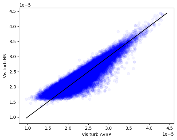
Note that the predictions y_pred_np and the test values y_test_np are divided by 10**5 here due to the scaling for the DL training. Well, that’s far away from perfect (an euphemism) but it will be good enough for this tutorial. Save the weights of your model now:
torch.save(model.state_dict(), 'model.pth')
You will now be able to use your model with PhyDLL. Note that you may also be interested in the AVBP dataloader created by none other than Fernando Gonzalez here.
4. Running your hybrid AI/AVBP solver
Copy/paste your run folder: cp -r RUN RUN_DL and enter the RUN_DL folder with: cd RUN_DL. Open the run.params and set LES_model = neuralnet. Move or copy/paste the model.pth created in the previous section in RUN_DL.
We now need to write the python script to load the model and send the fields from your DL model to AVBP. Open a main.py and copy/paste the following:
import numpy as np
import torch
from torch import nn
from phydll.phydll import PhyDLL

class NeuralNetwork(nn.Module):
    def __init__(self):
        n_inputs = 11
        n_outputs = 1
        n_neurones = 256
        super().__init__()
        self.linear_relu_stack = nn.Sequential(
            nn.Linear(n_inputs, n_neurones),
            nn.ReLU(),
            nn.Linear(n_neurones, n_neurones),
            nn.ReLU(),
            nn.Linear(n_neurones, n_neurones),
            nn.ReLU(),
            nn.Linear(n_neurones, n_neurones),
            nn.ReLU(),
            nn.Linear(n_neurones, n_neurones),
            nn.ReLU(),
            nn.Linear(n_neurones, n_outputs),
        )

    def forward(self, x):
        logits = self.linear_relu_stack(x)
        return logits

class MLP():

    def __init__(self, model_path):
        device = ("cuda" if torch.cuda.is_available() else "mps" if torch.backends.mps.is_available() else "cpu")
        print(f"Using {device} device")

        model = NeuralNetwork()
        model.load_state_dict(torch.load(model_path, weights_only=True, map_location=device))
        model.eval()
        self.model = model
        self.model.to(device)
        self.device = device

    def predict(self, fields):
        fields[0:9,:] /= 10**6
        fields[-1,:] *= 10**16

        X = torch.from_numpy(fields.T).float().to(self.device)

        with torch.no_grad():
            Y = self.model(X)

        Y = Y.cpu().detach().numpy().astype(np.float64)
        Y /= 10**5

        return Y.T

model_path = "model.pth"

def main():
    """
    Main coupling routine
    """
    phydll = PhyDLL(coupling_scheme="DS",
                    mesh_type="phymesh",
                    phy_nfields=11,
                    dl_nfields=1)
    # Temporal
    phydll.mpienv.glcomm.Barrier()
    use_temporal_loop = True

    model = MLP(model_path)

    if use_temporal_loop:
        phydll.set_predict_func(model.predict)
        phydll.temporal()
    else:
        while phydll.fsignal:
            phy_fields = phydll.receive_phy_fields()
            dl_fields = model.predict(phy_fields)
            phydll.send_dl_fields(dl_fields)

    # Finalize
    phydll.finalize()

if __name__ == "__main__":
    main()
NeuralNetwork is obviously the model we created. You might need to change it when you change your model. MLP is the class to manage this model. Note that in the predict we scale back to the original inputs/outputs due to the scaling we used for the DL model. Finally, in the main is executed the inference with AVBP. Note that in a future, you will have to change the phy_nfields and dl_fields according to your case.
This script might not be the best (yes, I am not perfect, sorry about that !). You can however find examples of python scripts for your models in phydll/scripts. In these scripts, there are methods like set_gpus that I do not master (I told you that I was not perfect!) so up to you to investigate this.
PhyDLL also relies on a phydll.yml for various parameters. So open a file named phydll.yml and copy/paste the following:
Output:
    debug_level : 3

Coupling:
  coupling_frequency : 1
  save_fields_frequency : 1        # (optional, default=0) Frequency to save exchanged fields in ./cwipi
The debug_level indicates the verbosity, the coupling_frequency is the frequence of coupling between AVBP and the DL fields, and the save_fields_frequency is the frequency to save the fields sent and received by PhyDLL.
Almost there ! If you are on Kraken, open a script that we name batch_job and copy paste the following:
#!/bin/bash
#SBATCH --job-name=first_run
#SBATCH --partition=debug
#SBATCH --nodes=1
#SBATCH --ntasks-per-node=36
#SBATCH --time=00:02:00
#SBATCH --output=output_test.o
#SBATCH --error=error_test.e
#SBATCH --exclusive

# LOAD MODULES ##########
module purge
module load avbp
module list
#########################
exec="/path/to/your/avbp/exec"

# NUMBER OF TASKS #######
export PHY_TASKS_PER_NODE=35
export DL_TASKS_PER_NODE=1
export TASKS_PER_NODE=$(($PHY_TASKS_PER_NODE + $DL_TASKS_PER_NODE))
export NP_PHY=$(($SLURM_NNODES * $PHY_TASKS_PER_NODE))
export NP_DL=$(($SLURM_NNODES * $DL_TASKS_PER_NODE))
#########################

# EXTRA COMMANDS ########
source /path/to/your/virtual/environment/bin/activate
#########################

# ENABLE PHYDLL #########
export ENABLE_PHYDLL=TRUE
#########################

# PLACEMENT FILE ########
python $PHYDLL_DIR/scripts/placement4mpmd.py --Run impi --NpPHY $NP_PHY --NpDL $NP_DL
#########################

# MPMD EXECUTION ########
mpirun -l --machinefile machinefile_$SLURM_NNODES-$NP_PHY-$NP_DL -np $NP_PHY $exec : -np $NP_DL python main.py
#########################
If you are on Calypso and planning to run on the grace partition, the script batch_job looks like this:
#!/bin/bash
#SBATCH --job-name=first_run
#SBATCH --gres=gpu:1
#SBATCH --partition=grace
#SBATCH --nodes=1
#SBATCH --ntasks-per-node=72
#SBATCH --time=00:01:00
#SBATCH --output=output_test.o
#SBATCH --error=error_test.e
#SBATCH --exclusive

# LOAD MODULES ##########
module purge
module load avbp/7.X_gcc124_ompi417
module list
#########################
exec="path/to/your/avbp/exec"

# NUMBER OF TASKS #######
export PHY_TASKS_PER_NODE=71
export DL_TASKS_PER_NODE=1
export TASKS_PER_NODE=$(($PHY_TASKS_PER_NODE + $DL_TASKS_PER_NODE))
export NP_PHY=$(($SLURM_NNODES * $PHY_TASKS_PER_NODE))
export NP_DL=$(($SLURM_NNODES * $DL_TASKS_PER_NODE))
#########################

# ENABLE PHYDLL #########
export ENABLE_PHYDLL=TRUE
#########################

# MPMD EXECUTION ########
mpirun -mca coll ^ucc --tag-output -np $NP_PHY $exec : -np $NP_DL singularity exec --nv -B /scratch/softs/local_arm/singularity/images/pytorch25.02.sif /path/to/your/virtual/environment/bin/python main.py

#########################
Note that on Calypso, there is no machinefile or rankfile involved as I did not manage to make it run with. Obviously, in both cases, you will need to change the path/to/your/avbp/exec and path/to/your/virtual/environment/ accordingly. These scripts can also be generated with PhyDLL like here.
You are now ready to submit your job:
sbatch batch_job
If everything went well, you normally should have at the end of output_test.o the line: (PhyDLL) -----> Finalizing. If that’s not the case … oh dear ! Well, I assume that you have this line. You can now inspect your two solutions: the one generated with Smagorinsky and the one generated by your DL model. Open paraview on the machine (once again, if you do not know how to do it, have a look at the intranet of CSG here and select the corresponding machine). Load your two solutions: RUN/solut_00000002.h5 and RUN_DL/solut_00000002.h5. Personnally, side by side, that looks something like this:
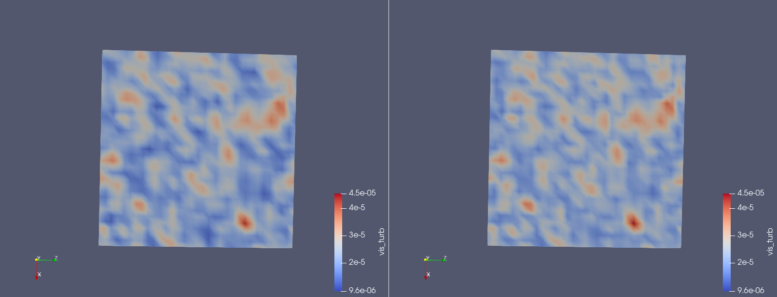
On the left, you have the viscosity turbulent computed with Smagorinsky and on the right, you have the one computed with the DL model. They are pretty similar in the end.
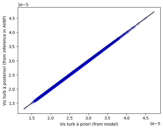
You can also check if your a priori inference is the same as your posteriori inference. In your jupyter notebook, copy/paste the following:
import torch
import h5py
import numpy as np

from torch import nn
from matplotlib import pyplot as plt

# We select the device
device = (
    "cuda"
    if torch.cuda.is_available()
    else "mps"
    if torch.backends.mps.is_available()
    else "cpu"
)
print(f"Using {device} device")

# We create again the same model
class NeuralNetwork(nn.Module):
    def __init__(self):
        n_inputs = 11
        n_outputs = 1
        n_neurones = 256
        super().__init__()
        self.linear_relu_stack = nn.Sequential(
            nn.Linear(n_inputs, n_neurones),
            nn.ReLU(),
            nn.Linear(n_neurones, n_neurones),
            nn.ReLU(),
            nn.Linear(n_neurones, n_neurones),
            nn.ReLU(),
            nn.Linear(n_neurones, n_neurones),
            nn.ReLU(),
            nn.Linear(n_neurones, n_neurones),
            nn.ReLU(),
            nn.Linear(n_neurones, n_outputs),
        )

    def forward(self, x):
        logits = self.linear_relu_stack(x)
        return logits

model = NeuralNetwork()
model.load_state_dict(torch.load('RUN_DL/model.pth', weights_only=True, map_location=device))
model.to(device)

# A priori
solut_priori = "INIT/solut_00000001.h5"
with h5py.File(solut_priori, "r") as solut:
    grad_ux = solut["Additionals"]["grad_ux"][:] / 10**6
    grad_uy = solut["Additionals"]["grad_uy"][:] / 10**6
    grad_uz = solut["Additionals"]["grad_uz"][:] / 10**6
    grad_vx = solut["Additionals"]["grad_vx"][:] / 10**6
    grad_vy = solut["Additionals"]["grad_vy"][:] / 10**6
    grad_vz = solut["Additionals"]["grad_vz"][:] / 10**6
    grad_wx = solut["Additionals"]["grad_wx"][:] / 10**6
    grad_wy = solut["Additionals"]["grad_wy"][:] / 10**6
    grad_wz = solut["Additionals"]["grad_wz"][:] / 10**6
    rho = solut["GaseousPhase"]["rho"][:]
    volw = solut["Additionals"]["volw"][:] * 10**16

x_prio = np.c_[grad_ux, grad_uy, grad_uz, grad_vx, grad_vy, grad_vz, grad_wx, grad_wy, grad_wz, rho, volw]
x_prio = torch.from_numpy(x_prio).float().to(device)

model.eval()
with torch.no_grad():
    y_prio = model(x_prio)
y_prio_np = y_prio.cpu().detach().numpy() / 10**5

# A posteriori
solut_posteriori = "RUN_DL/SOLUT/solut_00000002.h5"
with h5py.File(solut_posteriori, "r") as solut:
    y_post_np = solut["Additionals"]["vis_turb"][:]

print(y_prio_np.shape, y_post_np.shape)

min_y = np.min(np.r_[y_prio_np.flatten(), y_post_np])
max_y = np.max(np.r_[y_prio_np.flatten(), y_post_np])

plt.scatter(y_prio_np, y_post_np, color="blue", alpha=0.05)
plt.plot([min_y, max_y], [min_y, max_y], "k")
plt.xlabel("Vis turb à priori (from model)")
plt.ylabel("Vis turb à posteriori (from inference in AVBP)")
Personnally, I had:
You managed to reach this point ! Virtual high five ! You deserve it ! Scream to the world that you managed to make a coupling between AVBP and your DL model with PhyDLL ! Now, it is up to you to make your own couplings between AVBP and DL models.