Disclaimer : This tutorial is done using the software AVBP, a Cerfacs software available for academic research by requesting a Non Disclosure Agreement . See https://avbp-wiki.cerfacs.fr/ for more information on the AVBP software.
In this tutorial, we will see how to use PhyDLL to perform an online learning of an AVBP simulation. With this approach, the Deep Learning (DL) model will be trained at the same time as the AVBP simulation goes on. Compared to the offline learning where the model is trained with all the data available, the online learning is useful for applications where it is impossible to store the solutions to train the model or when you want your model to adapt to recent trends (e.g. stock market price).
In order to be able to perform this tutorial, please do the steps 0. and 1. of this previous tutorial. For the step 0, you will need to use the PhyDLL branch online_learning_v0.1:
cd phydll
git checkout online_learning_v0.1
If you are too lazy to do the step 1. for AVBP (which I would completely understand !) or you do not want to be bothered too much with Fortran (which once again I would completely understand !), you can start back from the tuto_phydll branch:
cd avbp
git checkout tuto_phydll
1. Test case
As in the aforementioned tutorial, we will take as a test case the decaying Homogeneous Isotropic Turbulence (HIT) with the Smagorinsky LES model. But this time, we will try to fit a model on the total Turbulent Kinetic Energy (TKE) given by:
whre \(k\) is the TKE, \(u^\prime\), \(v^\prime\) and \(w^\prime\) respectively represent the fluctuations of the velocity in the \(x\), \(y\) and \(z\) directions:
The \(\bar{.}\) represents the spatial mean of the quantity.
You can find the test case here. Download it, and set in RUN/run.params the simulation_end_iteration to 1000.
Run the case. If everything went well, you will have 1000 solutions in your SOLUT folder. We can use it to build the TKE with Python. Run in a jupyter notebook or in a Python program where you can have a graphical output:
import numpy as np
from matplotlib import pyplot as plt
import h5py
from pathlib import Path

# We build the turnover time.
L = 1.3900e-04 * 2
init_solut = "INIT/init_tetra.h5"

with h5py.File(init_solut, "r") as solut:
    rho = solut["GaseousPhase"]["rho"][:]
    u = solut["GaseousPhase"]["rhou"][:] / rho
    v = solut["GaseousPhase"]["rhov"][:] / rho
    w = solut["GaseousPhase"]["rhow"][:] / rho

    u_prime = u - np.mean(u)
    v_prime = v - np.mean(v)
    w_prime = w - np.mean(w)

    u_rms = np.sqrt(np.mean(u_prime**2 + v_prime**2 + w_prime**2) / 3)

t_turn = L / u_rms

# We build the TKE
folder = Path("RUN/SOLUT/")
h5_files = sorted(folder.glob("*.h5"))

for h5_file in h5_files[:]:
    # We exclude last_solution.h5 from the solutions found in SOLUT
    if "last_solution.h5" in h5_file.name:
        h5_files.remove(h5_file)

t_list = []
k_rms_list = []

for h5file in h5_files:
    with h5py.File(h5file, "r") as solut:
        t = solut["Parameters"]["dtsum"][:]
        rho = solut["GaseousPhase"]["rho"][:]
        u = solut["GaseousPhase"]["rhou"][:] / rho
        v = solut["GaseousPhase"]["rhov"][:] / rho
        w = solut["GaseousPhase"]["rhow"][:] / rho

        test_u = solut["HITgas"]["var_u"]

        u_prime = u - np.mean(u)
        v_prime = v - np.mean(v)
        w_prime = w - np.mean(w)

        k = 0.5 * np.mean(u_prime**2 + v_prime**2 + w_prime**2)
        t_list.append(t/t_turn)
        k_rms_list.append(k)

# Plot
plt.figure()
plt.plot(t_list, k_rms_list)
plt.ylabel("k")
plt.xlabel(r"t/${\tau}$")
plt.show()
Adapt the init_solut and the folder accordingly.
Normally, you should have something like this:
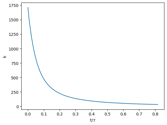
\(t\) is the time and \(\tau\) represents the turnover time given by:
where \(L\) is a characteristic length that we take here as the dimension of the domain and \(U\) a characteristic velocity that we define here as the root mean square of the velocity fluctuations:
2. Offline learning
In this tutorial, we will compare the online learning approach with an overfitted DL model built through offline learning. Thus, we will first build a DL model with PyTorch.
Of course the output of our model will be the TKE ! The inputs will be \(u\), \(v\), \(w\) in the whole domain.
First, we need to build a custom dataset with PyTorch with the corresponding inputs/outputs pairs. You can do that with the following script:
import h5py
import numpy as np
import torch

from torch.utils.data import Dataset
from pathlib import Path

class CustomDatasetMLP(Dataset):
    def __init__(self, folder):

        # We find the .h5 in the folder and sort them.
        folder = Path(folder)
        solutions = sorted(folder.glob("*.h5"))

        # We delete the "last_solution.h5" and find the number of points.
        for solution in solutions[:]:
            if "last_solution.h5" in solution.name:
                with h5py.File(solution, "r") as solut:
                    N = len(solut["GaseousPhase"]["rho"][:])
                solutions.remove(solution)

        self.inputs = np.zeros((len(solutions), 3, N))
        self.outputs = np.zeros((len(solutions), 1))

        for i, solution in enumerate(solutions):
            with h5py.File(solution, "r") as solut:
                rho = solut["GaseousPhase"]["rho"][:]
                u = solut["GaseousPhase"]["rhou"][:] / rho
                v = solut["GaseousPhase"]["rhov"][:] / rho
                w = solut["GaseousPhase"]["rhow"][:] / rho

                u_prime = u - np.mean(u)
                v_prime = v - np.mean(v)
                w_prime = w - np.mean(w)

                k = 0.5 * np.mean(u_prime**2 + v_prime**2 + w_prime**2)

                self.inputs[i,0,:] = u / 100
                self.inputs[i,1,:] = v / 100
                self.inputs[i,2,:] = w / 100

                self.outputs[i,:] = k

        self.inputs = torch.from_numpy(self.inputs).float()
        self.outputs = torch.from_numpy(self.outputs).float()

    def __len__(self):
        return len(self.inputs)

    def __getitem__(self, idx):
        u = self.inputs[idx, 0, :]
        v = self.inputs[idx, 1, :]
        w = self.inputs[idx, 2, :]

        velocity = torch.cat([u, v, w], dim=0)
        return velocity, self.outputs[idx]
Note that the inputs have been divided by 100 to stabilize the DL training.
The CustomDatasetMLP object is initialized with your SOLUT folder path:
folder = "RUN/SOLUT"
dataset = CustomDatasetMLP(folder)
Like in the previous PhyDLL tutorial, we will use a classical Multi-Layers Perceptron (MLP):
from torch import nn

class NeuralNetwork(nn.Module):
    def __init__(self):
        n_inputs = 107811
        n_outputs = 1
        n_neurones = 256
        super().__init__()
        self.linear_relu_stack = nn.Sequential(
            nn.Linear(n_inputs, n_neurones),
            nn.ReLU(),
            nn.Linear(n_neurones, n_neurones),
            nn.ReLU(),
            nn.Linear(n_neurones, n_neurones),
            nn.ReLU(),
            nn.Linear(n_neurones, n_neurones),
            nn.ReLU(),
            nn.Linear(n_neurones, n_neurones),
            nn.ReLU(),
            nn.Linear(n_neurones, n_outputs),
        )

    def forward(self, x):
        logits = self.linear_relu_stack(x)
        return logits
We can finally perform the training of this model:
import copy
from torch.utils.data import DataLoader

dataloader = DataLoader(dataset, batch_size=256)

device = (
    "cuda"
    if torch.cuda.is_available()
    else "mps"
    if torch.backends.mps.is_available()
    else "cpu"
)
print(f"Using {device} device")

model = NeuralNetwork().to(device)
print(model)

learning_rate = 1e-3
loss_fn = nn.MSELoss()
optimizer = torch.optim.Adam(model.parameters(), lr=learning_rate)

def train(dataloader, model, loss_fn, optimizer):
    size = len(dataloader.dataset)
    model.train()
    running_loss = 0.0

    for batch, (X, y) in enumerate(dataloader):
        X, y = X.to(device), y.to(device)

        # Compute prediction error
        pred = model(X)
        loss = loss_fn(pred, y)

        # Backpropagation
        loss.backward()
        optimizer.step()
        optimizer.zero_grad()

        if batch % 100 == 0:
            loss, current = loss.item(), (batch + 1) * len(X)
            print(f"loss: {loss:>7f}  [{current:>5d}/{size:>5d}]")

    epoch_loss = running_loss / size  # Moyenne de la perte
    return epoch_loss

def evaluate(dataloader, model, loss_fn):
    model.eval()
    running_loss = 0.0
    size = len(dataloader.dataset)

    with torch.no_grad():
        for X, y in dataloader:
            X, y = X.to(device), y.to(device)
            pred = model(X)
            loss = loss_fn(pred, y)
            running_loss += loss.item() * X.size(0)

    epoch_loss = running_loss / size
    return epoch_loss


epochs = 100
timely_loss_fcn = []
best_loss = float('inf')

for t in range(epochs):
    print(f"Epoch {t+1}\n-------------------------------")
    train(dataloader, model, loss_fn, optimizer)
    epoch_loss = evaluate(dataloader, model, loss_fn)
    timely_loss_fcn.append(epoch_loss)
    print(f"Epoch {t+1} average loss: {epoch_loss:.6f}")

    if epoch_loss < best_loss:
        best_loss = epoch_loss
        best_state_dict = copy.deepcopy(model.state_dict())
print("Done!")
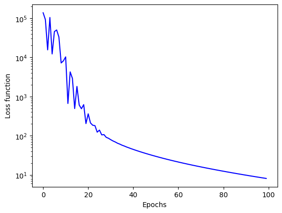
We can then plot the timely loss function:
from matplotlib import pyplot as plt

plt.figure()
plt.plot(np.arange(epochs), timely_loss_fcn, "b")
plt.xlabel("Epochs")
plt.ylabel("Loss function")
plt.yscale("log")
plt.show()
which should give you something like this:
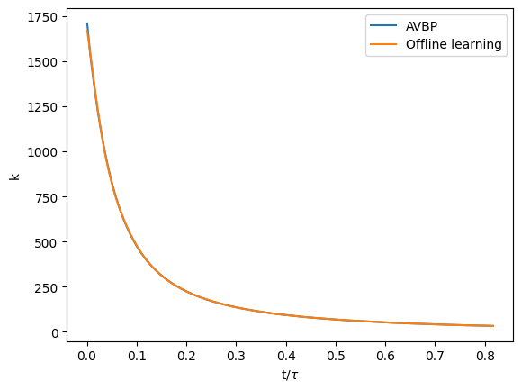
We can also compare with the real AVBP solutions. For that, you will need the t_turn, the t_list and k_rms_list given in Sec. 1.
Once you have it, you can run the following program to plot the TKE for both AVBP and your offline model:
y_offline = []

model.eval()

for i in range(0, len(dataset.inputs)):
    X, Y = dataset.__getitem__(i)
    X = X.to(device)
    with torch.no_grad():
        y = model(X)
    y = y.cpu().detach().numpy()
    y_offline.append(y)

plt.figure()
plt.plot(t_list, k_rms_list, label="AVBP")
plt.plot(t_list, y_offline, label="Offline learning")
plt.ylabel("k")
plt.xlabel(r"t/${\tau}$")
plt.legend()
plt.show()
which personnaly gave me:
Since it will be useful later, we can also plot the relative error between your model and the real AVBP simulations:
plt.figure()
plt.plot(t_list, np.abs(np.array(k_rms_list) - np.array(y_offline).ravel()) / np.array(k_rms_list), label="Offline")
plt.ylabel(r"$\epsilon$")
plt.xlabel(r"t/${\tau}$")
plt.legend()
plt.show()
which personnally gave me:
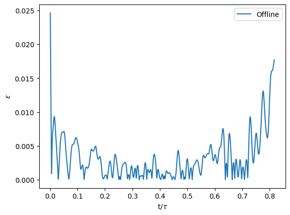
Well, that is not so bad, as we have an error inferior to \(2.5\%\) everywhere ! Feel free to explore the batch_size, the learning rate and the number of epochs to check how reacts the model ! But for now, we will save the weights that we have:
torch.save(model.state_dict(), 'model_offline.pth')
3. Online learning
We can finally move on to the online learning part.
3.1 Implementation of the fields to send in AVBP
This step will be basically the same as the step 2.1 of the AVBP/PhyDLL tutorial but simpler ! Hallelujah ! (tough word to write, I had to google that to check the orthography)
If it is not already done, you will have to create a file named neuralnet_fields_to_send.f90 in SOURCES/MAIN and copy/paste the following code:
!--------------------------------------------------------------------------------------------------
!     Copyright (c) CERFACS (all rights reserved)
!--------------------------------------------------------------------------------------------------


!--------------------------------------------------------------------------------------------------
!     MODULE mod_neuralnet_fields_to_send
!>    @brief   Set the fields to send from AVBP to your Deep Learning model through PhyDLL
!!    @details Set the fields to send from AVBP to your Deep Learning model through PhyDLL
!!    @authors A. Larroque
!!    @date    2025-02-25
!--------------------------------------------------------------------------------------------------
MODULE mod_neuralnet_fields_to_send

  USE mod_param_defs

  CONTAINS

    SUBROUTINE neuralnet_set_fields_to_send ( grid )

    USE mod_grid,                    ONLY: grid_t
    USE mod_timers,                  ONLY: timer_start, timer_stop
    USE mod_input_param_defs,        ONLY: itimers
    USE mod_misc_defs,               ONLY: avbpdl_timer_send_pre
#ifdef PHYDLL
    USE phydll,                      ONLY: phydll_set_phy_field, phydll_send_phy_fields
    USE mod_parallel_defs,           ONLY: enable_phydll
#endif

    IMPLICIT NONE

!   IN/OUT
    TYPE(grid_t) :: grid

    CALL timer_start ( avbpdl_timer_send_pre, itimers )

#ifdef PHYDLL
    IF (enable_phydll == YES_) THEN
      CALL phydll_set_phy_field(field=grid%data_n%w(1,:), label="rho", index=1)
      CALL phydll_set_phy_field(field=grid%data_n%w(2,:), label="rhou", index=2)
      CALL phydll_set_phy_field(field=grid%data_n%w(3,:), label="rhov", index=3)
      CALL phydll_set_phy_field(field=grid%data_n%w(4,:), label="rhow", index=4)
      CALL phydll_set_phy_field(field=grid%data_n%x(1,:), label="x", index=5)
      CALL phydll_set_phy_field(field=grid%data_n%x(2,:), label="y", index=6)
      CALL phydll_set_phy_field(field=grid%data_n%x(3,:), label="z", index=7)
      CALL phydll_send_phy_fields(loop=.true., ol=.true.)
    END IF
#endif

    CALL timer_stop ( avbpdl_timer_send_pre, itimers )

  END SUBROUTINE neuralnet_set_fields_to_send

END MODULE mod_neuralnet_fields_to_send
Note that the only difference with the other tutorial (except that this function is simpler since we do not compute the gradients) is the ol=.true. in phydll_send_phy_fields. This is to specify that we are in a online learning framework so that AVBP will not need to wait later to receive fields from the Python program.
Note that the first fields sent are the density \(\rho\) and the conservative variables of Navier Stokes equations: \(\rho u\), \(\rho v\) and \(\rho w\). We will then compute again the velocity fields with these four variables. The last fields are the coordinates of the points \(x\), \(y\), and \(z\). This will be needed later as the fields sent through PhyDLL are not stored in the same order as it is in the mesh mesh.h5. So to compare our model, with the data issued from the offline learning, we will need the coordinates to reorder the inputs of the model.
Once again, if it is not already done, open SOURCES/MAIN/compute.f90, replace at the beginning of the subroutine compute:
USE mod_efcy_neuralnet, ONLY: efcy_neuralnet_set_fields_to_send
for
USE mod_neuralnet_fields_to_send, ONLY: neuralnet_set_fields_to_send
and change at the beginning the paragraph:
! ----------------------------------------------------------------------
! Sends species-based progress variable to Python (AVBP-DL)
! ----------------------------------------------------------------------
    IF ( kstage==1 .AND. enable_phydll==YES_ ) THEN
      IF ( using_acc ) THEN
        message = "kstage==1 .AND. enable_phydll==YES_ not supported by with openACC"
        CALL print_error_and_quit ( err_routine=routine, err_message=message )
      END IF
      CALL efcy_neuralnet_set_fields_to_send ( grid )
      CALL send_coupling ( coupling(avbpdl) )
    END IF
for
! ----------------------------------------------------------------------
! Sends species-based progress variable to Python (PhyDLL)
! ----------------------------------------------------------------------
    IF ( kstage==1 .AND. enable_phydll==YES_ ) THEN
      IF ( using_acc ) THEN
        message = "kstage==1 .AND. enable_phydll==YES_ not supported by with openACC"
        CALL print_error_and_quit ( err_routine=routine, err_message=message )
      END IF
      CALL neuralnet_set_fields_to_send ( grid )
    END IF
That’s it, your fields are ready to be sent from AVBP to your DL model for your online learning.
3.2 The Python program
Copy your RUN folder to RUN_DL and enter in the new folder created. Open the run.params and set the save_solution to no.
Now, open a file named phydll.yml and copy/paste the following:
Output:
    debug_level : 3

Coupling:
  coupling_frequency : 1
  save_fields_frequency : 1        # (optional, default=0) Frequency to save exchanged fields in ./cwipi
Finally, we can create the python program in charge to train the model on-the-fly. Open a file named main.py and copy/paste the following:
import numpy as np
from phydll.phydll import PhyDLL
import h5py
import numpy as np
import torch

from torch.utils.data import Dataset, DataLoader
from torch import nn
import copy
from pathlib import Path

class CustomDatasetMLP(Dataset):
    def __init__(self, u_list, v_list, w_list):
        u = np.array(u_list)
        v = np.array(v_list)
        w = np.array(w_list)

        u_prime = u - np.mean(u, axis=1).reshape(-1,1)
        v_prime = v - np.mean(v, axis=1).reshape(-1,1)
        w_prime = w - np.mean(w, axis=1).reshape(-1,1)

        k = 0.5 * np.mean(u_prime**2 + v_prime**2 + w_prime**2, axis=1)

        self.inputs = np.zeros((u.shape[0], 3, u.shape[1]))
        self.outputs = np.zeros((u.shape[0], 1))

        self.inputs[:,0,:] = u / 100
        self.inputs[:,1,:] = v / 100
        self.inputs[:,2,:] = w / 100
        self.outputs[:,:] = k.reshape(-1,1)

        self.inputs = torch.from_numpy(self.inputs).float()
        self.outputs = torch.from_numpy(self.outputs).float()

    def __len__(self):
        return len(self.inputs)

    def __getitem__(self, idx):
        u = self.inputs[idx, 0, :]
        v = self.inputs[idx, 1, :]
        w = self.inputs[idx, 2, :]

        velocity = torch.cat([u, v, w], dim=0)
        return velocity, self.outputs[idx]


class NeuralNetwork(nn.Module):
    def __init__(self):
        n_inputs = 107811
        n_outputs = 1
        n_neurones = 256
        super().__init__()
        self.linear_relu_stack = nn.Sequential(
            nn.Linear(n_inputs, n_neurones),
            nn.ReLU(),
            nn.Linear(n_neurones, n_neurones),
            nn.ReLU(),
            nn.Linear(n_neurones, n_neurones),
            nn.ReLU(),
            nn.Linear(n_neurones, n_neurones),
            nn.ReLU(),
            nn.Linear(n_neurones, n_neurones),
            nn.ReLU(),
            nn.Linear(n_neurones, n_outputs),
        )

    def forward(self, x):
        logits = self.linear_relu_stack(x)
        return logits

device = (
    "cuda"
    if torch.cuda.is_available()
    else "mps"
    if torch.backends.mps.is_available()
    else "cpu"
)

print(f"Using {device} device")

model = NeuralNetwork().to(device)
print(model)

learning_rate = 1e-3
loss_fn = nn.MSELoss()
optimizer = torch.optim.Adam(model.parameters(), lr=learning_rate)

def train(dataloader, model, loss_fn, optimizer):
    size = len(dataloader.dataset)
    model.train()
    running_loss = 0.0

    for batch, (X, y) in enumerate(dataloader):
        X, y = X.to(device), y.to(device)

        # Compute prediction error
        pred = model(X)
        loss = loss_fn(pred, y)

        # Backpropagation
        loss.backward()
        optimizer.step()
        optimizer.zero_grad()

        if batch % 100 == 0:
            loss, current = loss.item(), (batch + 1) * len(X)
            print(f"loss: {loss:>7f}  [{current:>5d}/{size:>5d}]")


def evaluate(dataloader, model, loss_fn):
    model.eval()
    running_loss = 0.0
    size = len(dataloader.dataset)

    with torch.no_grad():
        for X, y in dataloader:
            X, y = X.to(device), y.to(device)
            pred = model(X)
            loss = loss_fn(pred, y)
            running_loss += loss.item() * X.size(0)

    epoch_loss = running_loss / size
    return epoch_loss


def find_argmin_dataset(dataset, model):
    model.eval()
    u = dataset.inputs[:, 0, :]
    v = dataset.inputs[:, 1, :]
    w = dataset.inputs[:, 2, :]

    X = torch.cat([u,v,w], dim=1)
    X = X.to(device)

    with torch.no_grad():
        Y = model(X)

        error = torch.abs(Y - dataset.outputs.to(device))

    idx_min = torch.argmin(error)

    return idx_min


def main():
    """
    Main coupling routine
    """
    phydll = PhyDLL(coupling_scheme="DS",
                    mesh_type="phymesh",
                    phy_nfields=7,
                    dl_nfields=0)
    epochs = 1
    best_loss = float('inf')
    c = 0
    timely_loss_fcn = []
    u_list = []
    v_list = []
    w_list = []
    n_samples = 1
    batch_size = n_samples

    # Temporal
    phydll.mpienv.glcomm.Barrier()
    use_temporal_loop = False
    if use_temporal_loop:
        phydll.set_predict_func(your_predict_fct)
        phydll.temporal()
    else:
        while phydll.fsignal:
            phy_fields = phydll.receive_phy_fields()
            rho = phy_fields[0,:]
            u_list.append(phy_fields[1,:] / rho)
            v_list.append(phy_fields[2,:] / rho)
            w_list.append(phy_fields[3,:] / rho)

            if c == 0:
                x = phy_fields[4,:]
                y = phy_fields[5,:]
                z = phy_fields[6,:]
                coord = np.zeros((len(x), 3))
                coord[:,0] = x
                coord[:,1] = y
                coord[:,2] = z
                np.save("coordinates", coord)

            dataset = CustomDatasetMLP(u_list, v_list, w_list)

            if len(u_list) > n_samples:
                idx_min = find_argmin_dataset(dataset, model)
                u_list.pop(idx_min)
                v_list.pop(idx_min)
                w_list.pop(idx_min)
                dataset.inputs = torch.cat([dataset.inputs[:idx_min,:,:], dataset.inputs[idx_min+1:,:,:]], dim=0)
                dataset.outputs = torch.cat([dataset.outputs[:idx_min,:], dataset.outputs[idx_min+1:,:]], dim=0)

            dataloader = DataLoader(dataset, batch_size=batch_size)

            for t in range(epochs):
                print(f"Epoch {t+1}\n-------------------------------")
                train(dataloader, model, loss_fn, optimizer)
                epoch_loss = evaluate(dataloader, model, loss_fn)
                timely_loss_fcn.append(epoch_loss)

                if epoch_loss < best_loss:
                    best_loss = epoch_loss
                    torch.save(model.state_dict(), f"model_online_{n_samples}.pth")
                    print(f"MIN FOUND: {best_loss} at iteration : {c}")

            c += 1

    np.save(f"timely_loss_online_{n_samples}", np.array(timely_loss_fcn))

    # Finalize
    phydll.finalize()

if __name__ == "__main__":
    main()
Okay, that is a lot to take ! Take a deep breath to release the anxiety, and let me break it for you !
The first thing that you may notice is the CustomDatasetMLP is slightly different than the one that we used for the offline learning. The reason is that we here, we do not use the .h5 files but rather the fields directly sent by AVBP in an array.
As in the offline learning, we find the train function to train our model, the evaluate function to evaluate the loss and later keep the weights that minimize this loss, and finally the find_argmin_dataset function that you may wonder what it is for.
Let me explain it for you ! For this tutorial, we will use what we call a reservoir: we will store some solutions in the time in order to train our model. The size of this reservoir is determined by n_samples in the program. Thus, this find_argmin_dataset function will be in charge to determine which sample we must delete in the dataset when the size of the reservoir is exceeded with the new fields received. In order to determine which sample, we delete, we will use the Maximum Absolute Error (MAE):
where \(\hat{Y}\) is the prediction on the outputs of the model and \(Y\) the true outputs. The sample with the smallest MAE will be deleted from the dataset.
The rest of the program is classic as in other PhyDLL applications, except that instead of sending DL fields, we train our model in the main loop. For this reason, we set dl_fields = 0 in the PhyDLL object as we do not send DL fields to AVBP and there are no phydll.send_dl_fields().
Also, note that in the main loop, we keep the coordinates in coord and save them in a numpy format in order to rebuild later the model with the h5 files. Also, even if it will not be shown in this tutorial, the evolution of the loss function is also saved in a numpy format under the name timely_loss_function_{n_samples}.npy. Feel free to later plot them !
Okay, we hare ready to submit the job !
3.3 Run your job
In your RUN_DL folder, open a file named batch_job and copy/paste the following:
#!/bin/bash
#SBATCH --job-name=first_run
#SBATCH --partition=t4
#SBATCH --gres=gpu:1
#SBATCH --nodes=1
#SBATCH --ntasks-per-node=32
#SBATCH --time=00:10:00
#SBATCH --output=output_test.o
#SBATCH --error=error_test.e
#SBATCH --exclusive

# LOAD MODULES ##########
module list
#########################
exec="$AVBP_HOME/HOST/KRAKEN/BIN/AVBP_V7_dev.KRAKEN"

# NUMBER OF TASKS #######
export PHY_TASKS_PER_NODE=31
export DL_TASKS_PER_NODE=1
export TASKS_PER_NODE=$(($PHY_TASKS_PER_NODE + $DL_TASKS_PER_NODE))
export NP_PHY=$(($SLURM_NNODES * $PHY_TASKS_PER_NODE))
export NP_DL=$(($SLURM_NNODES * $DL_TASKS_PER_NODE))
#########################

# EXTRA COMMANDS ########
source /scratch/coop/larroque/python_venvs/phydll_venv/bin/activate
#########################

# ENABLE PHYDLL #########
export ENABLE_PHYDLL=TRUE
#########################

# PLACEMENT FILE ########
python /scratch/coop/larroque/softwares/GITLAB/PHYDLL/scripts/placement4mpmd.py --Run impi --NpPHY $NP_PHY --NpDL $NP_DL
#########################

# MPMD EXECUTION ########
mpirun -l --machinefile machinefile_$SLURM_NNODES-$NP_PHY-$NP_DL -np $NP_PHY $exec : -np $NP_DL python main.py
#########################
This script is an example to run on Kraken. Adapt it to your machine. Note that you can also use the script generator given by PhyDLL. Also, do not forget to change the paths mentioned in the script accordingly !
4. Comparison offline/online
In this tutorial, I ran the simulation for n_samples = 1, 5, 10, 20, 50, 100.
We can now exploit the results, the first step is to create a mapping between the coordinates of the .h5 files and the coordinates sent by PhyDLL:
import h5py
import numpy as np

# We have to shuffle the inputs so the coordinates sent by PhyDLL and in the .h5 are the sames
coord_phydll = np.load("RUN_DL_tuto/coordinates.npy")

with h5py.File("MESH/mesh_tetra.mesh.h5", "r") as mesh:
    x = mesh["Coordinates"]["x"][:]
    y = mesh["Coordinates"]["y"][:]
    z = mesh["Coordinates"]["z"][:]

coord_h5 = np.zeros((len(x), 3))
coord_h5[:,0] = x
coord_h5[:,1] = y
coord_h5[:,2] = z

x1_view = [tuple(row) for row in coord_phydll]
x2_view = [tuple(row) for row in coord_h5]


x2_dict = {val: i for i, val in enumerate(x2_view)}

idx = np.array([x2_dict[row] for row in x1_view])
Using the dataset and model created in Sec. 2, we can then reorder the coordinates in the .h5 files in order to create predictions with our different models:
n_samples_list = [1, 5, 10, 20, 50, 100]
y_online_list = []

for n_samples in n_samples_list:
    y_online = []

    model = NeuralNetwork()
    model.load_state_dict(torch.load(f"RUN_DL_tuto/model_online_{n_samples}.pth", weights_only=True, map_location=device))
    model.to(device)
    model.eval()

    for i in range(0, len(dataset)):
        inputs, Y = dataset.inputs[i], dataset.outputs[i]
        u = inputs[0, :]
        v = inputs[1, :]
        w = inputs[2, :]

        u = u[idx]
        v = v[idx]
        w = w[idx]

        X = torch.cat([u, v, w], dim=0)
        X = X.to(device)
        with torch.no_grad():
            y = model(X)
        y = y.cpu().detach().numpy()
        y_online.append(y)

    y_online_list.append(y_online)
We can then compare with the online learning. If you do not have it loaded, you can use the following program:
y_offline = []

model = NeuralNetwork()
model.load_state_dict(torch.load('model_offline.pth', weights_only=True, map_location=device))
model.to(device)
model.eval()

for i in range(0, len(dataset.inputs)):
    X, Y = dataset.__getitem__(i)
    X = X.to(device)
    with torch.no_grad():
        y = model(X)
    y = y.cpu().detach().numpy()
    y_offline.append(y)
We are now ready to plot the relative error for each model:
plt.figure()
plt.plot(t_list, np.abs(np.array(k_rms_list) - np.array(y_offline).ravel()) / np.array(k_rms_list), label="Offline")

for i, n_samples in enumerate(n_samples_list):
    plt.plot(t_list, np.abs(np.array(k_rms_list) - np.array(y_online_list[i]).ravel()) / np.array(k_rms_list), label=f"Online learning ({n_samples})")
plt.ylabel(r"$\epsilon$")
plt.xlabel(r"t/${\tau}$")
plt.legend()
plt.show()
which personnally gave me:
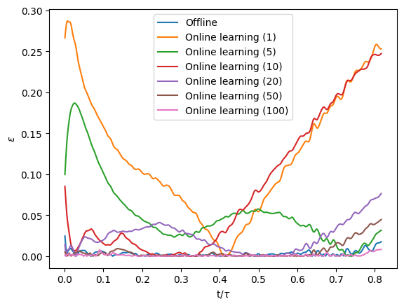
As we can see, with 1, 5, or 10 samples in our reservoir, large errors can be found at one extremity (or even both) of the curve. After investigation with the timely loss functions that we kept, it seems to be linked to how we saved the weights of the model. Indeed, we kept the weights that minimized the loss function during the whole simulation. So for 1 and 10 samples, the weights were kept at approximately half the simulation whereas for 5 samples, they were kept around the end of the simulation.
Anyways, we see that the accuracy of the model globally increases as we keep more samples in our reservoir and find pretty good results with 100 samples in our reservoir ! We can even compare the difference between the error found with the offline model and the one got through online learning with 100 samples:
plt.figure()
e_offline = np.abs(np.array(k_rms_list) - np.array(y_offline).ravel()) / np.array(k_rms_list)
e_online = np.abs(np.array(k_rms_list) - np.array(y_online_list[-1]).ravel()) / np.array(k_rms_list)
plt.plot(t_list, e_offline - e_online , "r")
plt.axhline(y=0, color='black', linestyle='--', linewidth=1)
plt.ylabel(r"$\epsilon_{offline} - \epsilon_{online}$")
plt.xlabel(r"t/${\tau}$")
plt.show()
which personally gave me:
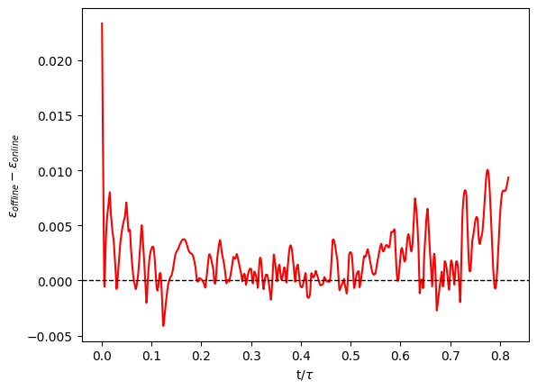
The online learning gave generally better results than the offline learning ! One hypothesis worth investigating to explain that would be that the online learning had in the end more “total epochs” since it was optimized each time it received fields. So it was more efficient to perform more optimization iterations than using a larger dataset for the model, especially due to the simple expression linking the velocities and the TKE.
But I leave that to you to check the veracity of this hypothesis and to investigate how reacts the online learning when you change the way you store the weights, the samples in the reservoir and parameters such as epochs, learning_rate and batch_size ;)
5. Final notes
With the online_learning_0.1 branch of PhyDLL, AVBP is supposed to run asynchronously of the training of your DL model. The fields will be sent in a buffer and the DL model will use them when it will be ready.
However, it may happen that your simulation runs much faster than your DL model and the buffer will be full. In that case, AVBP will wait for storage in the buffer to be available before going on the next iteration, hence slowing down the AVBP simulation.
If that’s a problem for you, you can increase the coupling_frequency of your phydll.yml to send less regularly fields to your DL model.
You can also design more elaborated stragies on the python side such as waiting to receive a certain number of samples before training your model.
A final possibility is to use the phydll_check_ready_signal_dl and phydll_recv_ready_signal_dl of the Fortran interface and the phydll_send_ready_signal on the Python side. phydll_recv_ready_signal_dl will wait in a non-blocking way the signal that the DL model is ready to receive fields, phydll_check_ready_signal_dl will check for this signal, and phydll_send_ready_signal will send the signal from the Python side that the DL model is now ready to receive fields. You can check a minimal example of this approach here. Note however that this approach may be conflictual with the coupling_iteration of the phydll.yml.
That’s it, you can go back to a normal activity !