
Context of these academical Benchmarks
![]()
SCALABLE must “achieve the scaling to unprecedented performance, scalability, and energy efficiency of an industrial LBM-based computational fluid dynamics (CFD) software.” The following four benchmarks highlights the numerical precision with an academical convection of a vortex, the turbulence modeling capacity with an academical turbulent channel, the aero-acoustic capabilities with the landing gear configuration and finally the assessment of both small and large physical phenomenon with the S2A car rig.
Convected vortex
The idea of this test case is to convect a two dimensional isentropic vortex in a bi-periodic domain. This benchmark is too simple for extensive HPC use however offers the advantage of being simple enough to evaluate weak scaling performance and basic non regression for an analytical flow. Such a vortex can be generated using the following function:
with \(\Gamma\) and \(R_c\) the circulation and vortex radius respectively. \(x_c\) and \(y_c\) correspond to the coordinates of the vortex center. Following this, both pressure and velocity local components can be expressed as follows:
The values and significance of the different parameters of the aforementioned expressions (as well as some mesh specifics) are defined in the following table:
| Convected Vortex Parameters | |
|---|---|
| Domain bounding box | -0.05 x 0.05 m |
| Resolution | 64x64 |
| Density | \(\rho_0\) = \(1.1608 Kg.m^3\) |
| Temperature | \(300 K\) |
| Pressure | \(P_0\) = 1 bar |
| Circulation | \(\Gamma\)= \(34.728 m^{2}.s^{-1}\) |
| Radius | \(R_c\) = 0.005 m |
| Convection Speed | \(U_0\) = \(170m.s^{-1}\) ; \(V_0\) = 0 |
You can download a Cerfacs Technical report giving more details on the initialization equations here.
As in LBM the streaming operator is aligned with the grid, a vortex convection from west to east is too simple , only one direction is really tested. Therefore a more challenging test case is a vortex convected back with an angle, exactly atan(1/10)/\(\pi\) x 180 = 5,71059314 (after 10 revolutions, the vortex should be back in the center). The only added difference expected from the aligned use case is a small velocity component to the Y direction (south to north) which is specified in the following table:
| Unaligned Convected Vortex | |
|---|---|
| Convection speed x | \(U_0\) = \(170 m.s^{-1}\) (Mach 0.5) |
| Convection speed y | \(V_0\)= \(17 m.s^{-1}\) |
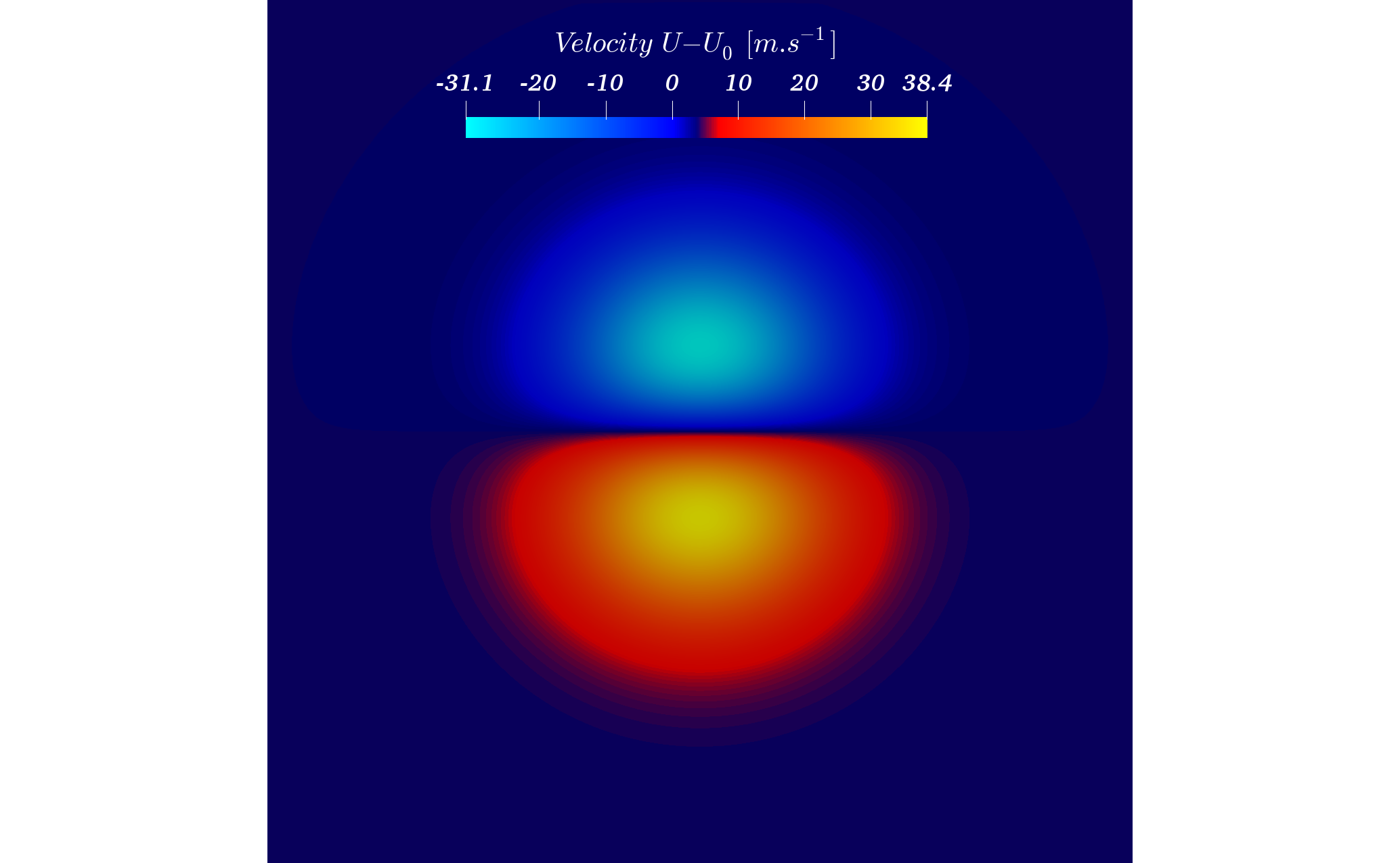
Longitudinal Velocity field of a Vortex convected by ProLB, 3rd turnaround.
Turbulent flow between two parallel plates
In order to carefully assess turbulence modeling capabilities, it’s important to start with cases where the analytical theory allows to be quantitative. The second academic test case is a classical turbulent flow in a channel composed of two parallel plates. This configuration is based on the Physics of Fluids article of Moser et al: Robert D. Moser, John Kim, and Nagi N. Mansour. “Direct numerical simulation of turbulent channel flow up to \(Re_{\theta}\)= 590”. In: Physics of Fluids 11.4 (1999), pp. 943—945. doi: 10.1063/1.869966. url: https://doi.org/10.1063/1.869966.
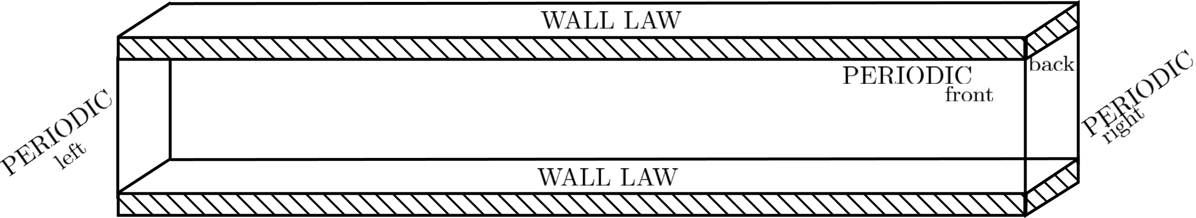
Standard configuration for a turbulent flow between parallel plates.
It consists of a three dimensional periodic channel with walls at the top and the bottom boundaries. A forcing term is applied on the pressure gradient in the normal direction in order to create and maintain the flow direction. The mesh and physical parameters are given in the following table.
| Turbulent flow between two parallel plates | |
|---|---|
| Shape LxHxW | \(\pi\) H/2 x H x 0.289 \(\pi\) H/2 |
| Dimensions LxHxW | 0,314 x 0,2 x 0,09 m |
| Resolution \(\Delta x\) | 0,001m |
| Resolution \(\Delta y\) | 0,001m |
| \(\Delta y^+\) | 5,44 |
| Cells | 5,652 Million tetrahedra (314x200x90) |
| Domain Height | H = 0.2m |
| Density | 1.1608 \(Kg.m^3\) |
| Temperature | 300 K |
| Pressure | \(10^{5}\) Pa |
| Bulk Reynolds | \(Re\) = 10 000 |
| Bulk Velocity | 1,61268091 \(m.s^{-1}\) |
| Skin Friction coef. | \(5.908e^{-3}\) |
| Wall Shear stress | \(\tau_w\) = \(8,92e^{-3}\) |
| Forcing term | 0,089179448 \(kg.m^{-2}.s^{-2}\) |
| Friction Reynolds | \(Re_{\tau}\) = 544 |
Lagoon Landing gear
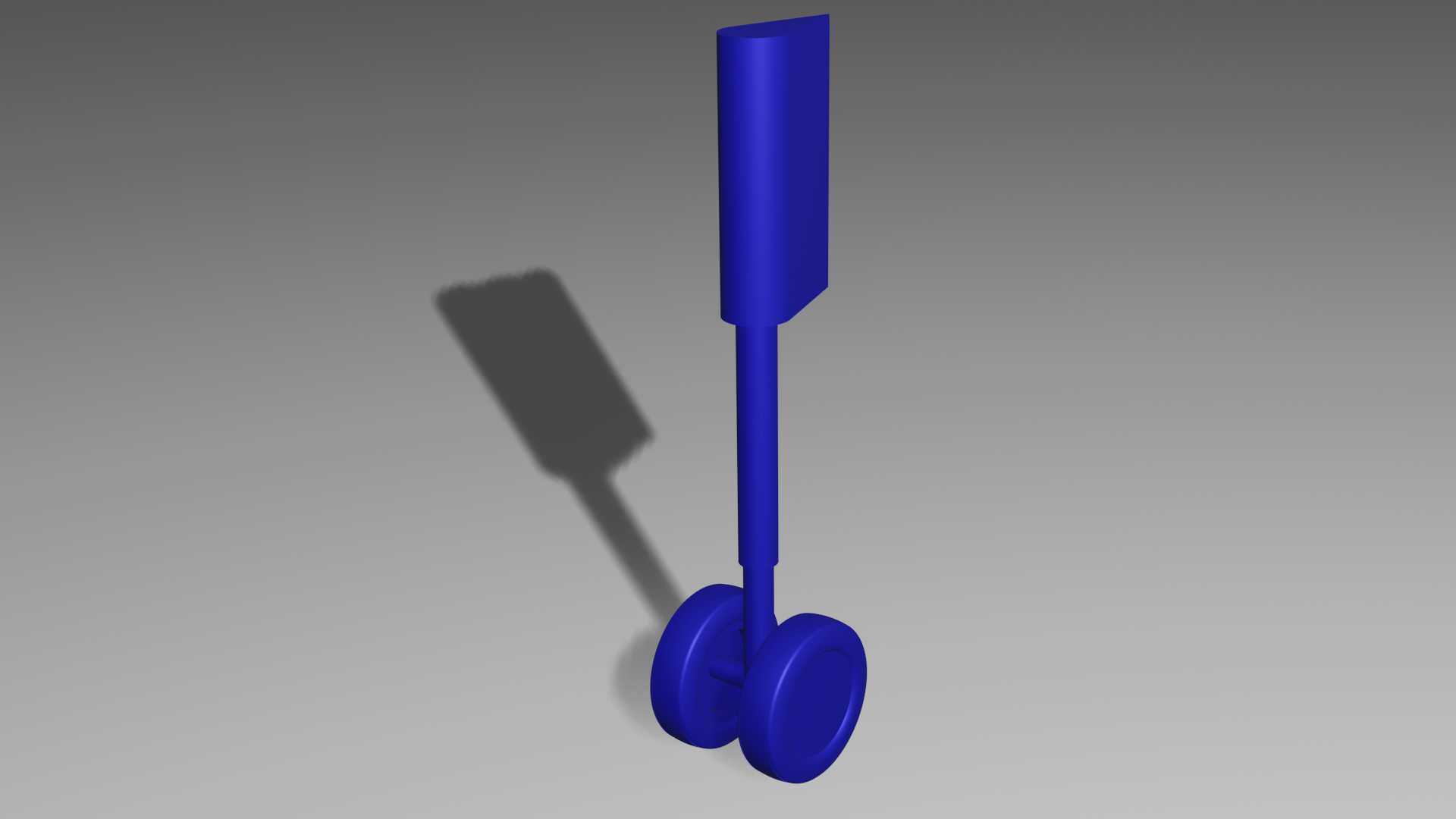
Lagoon landing gear geometry.
The third test case, and the first industrial application, follows the previous one as it focuses on testing 3D turbulent flows capabilities but in a more complex situation: a turbulent flow around a full landing gear. Called "lagoon", this test case has been largely used to benchmark various industrial and research codes and consist in a simplified deployed front landing gear from an Airbus plane in final approach operating conditions before landing. This configuration produces an interesting non-trivial flow and allows to assess both the aerodynamic and acoustic fields and can be compared them to a large experimental and numerical database for validation. The physical and numerical parameters of the case are described in the following table:
| Lagoon Parameters | |
|---|---|
| Reynolds number | \(1.59 e^{6}\) |
| Reference Length | 0.3 m |
| Pressure | 99447 Pa |
| Temperature | 293.15 K |
| Velocity | \(78.99 m.s^{-1}\) |
| Minimal mesh size | \(5 e^{-4}\) m |
S2A flow around a car
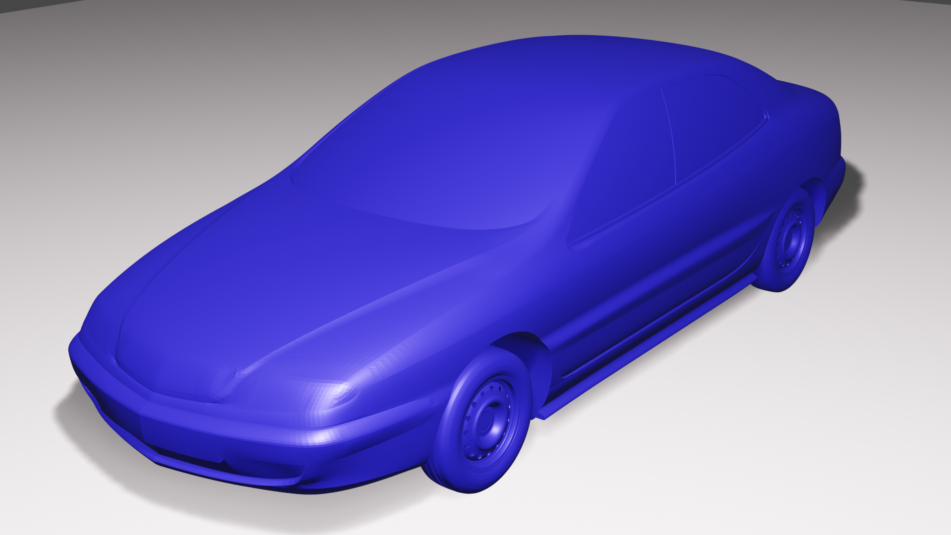
S2A car geometry.
The final test case consist in a modern sedan car placed inside a wind tunnel. Parameters for the simulation are described in the following Table:
| S2A Parameters | |
|---|---|
| Reynolds number | \(5.19 e^{6}\) |
| Reference Length | 1.7 m |
| Pressure | 101325 Pa |
| Temperature | 293 K |
| Velocity | \(45.83 m.s^{-1}\) |
| Minimal mesh size | \(25e^{-4}\) |