
Spaghetti code is a pejorative word used by readers that cannot figure out the code structure. The mental image of who does what is just too hard to get. We will see here how you can use Call graphs to deal with the refactoring of entangled spaghetti. (Si, questi sono bucatini…)
Getting started
The call graph is a log of the different routines calling each other. It traces what the reader would look if he were to perform an exhaustive read in the chronological order.
 An execution call graph generated for a simple computer program in Python.
Tools and litterature are abundant on the topic This document details some pratical applications of callgraphs in Python from the point of view of an end-user.
Execution vs static analysis
We oppose here two approches:
In an execution callgraph, the graph is generated through the actual execution of the target program. Therefore, the result is focused on -or limited to- a single set of features involved by this execution. Use execution callgraph when you want to understand or streamline one process in the software.
On the contrary, the static callgraph tries to map all the combinations between the possible processes in a software, using a static analysis (reading the sources without execution). Use static callgraphs to get a global overview of what the code can do and how well connected it is.
Execution callgraph generation
In python there are several utilities for this task. There is in particular a family of pycallgraph packages such as:
- pycallgraph2 (not tested here)
- pycallgraph3
All are installable from the PyPI index.
Unfortunately, to the author knowledge, none is emerging as “the” reference.
For example as we are writing these lines, pycallgraph2 is forked 302 times, last edition in 2019, july, and pycallgraph3 repository link on Pypi is broken.
Getting started with pycallgraph3
To visualize results, we will use a non-python resource : Graphviz. Read the download section to find your way out.
At CERFACS most of the user will get it on OSX using
brew install graphviz
(Beware, brew can mess up your Python installation by upgrading it). This tutorial will use pycallgraph3, which we install this way:
pip install pycallgraph3
We will create a small script to investigate a target main function, for the example run_cli().
What are the inputs needed to create a call graph?
We will use function call_graph_filtered() as a wrapper for pycallgraph3.
In the arguments we find the target function cli_run - Note that there is no () since we pass the function, not its result-.
The argument custom_include is narrowing the callgraph to a limited set of packages. It is highly recommended to limit the depth of the packages you want to trace. Indeed, without any limitation, python callgraph can become extremely large.
#!/usr/bin/env python
(...)
from oms.plan40.run_plan40 import cli_run

call_graph_filtered(
    cli_run,
    custom_include=["oms.*", "pyavbp.*"],# "kokiy.*", "ms_thermo.*", "arnica.*"],
)
Creating the wrapper call_graph_filtered()
The wrapper function call_graph_filtered() is defined as the following.
from pycallgraph3 import PyCallGraph
from pycallgraph3 import Config
from pycallgraph3 import GlobbingFilter
from pycallgraph3.output import GraphvizOutput

def call_graph_filtered(
        function_,
        output_png="call_graph_png",
        custom_include=None

    ):
    """A call graph generator filtered"""
    config = Config()
    config.trace_filter = GlobbingFilter(
        include=custom_include)
    graphviz = GraphvizOutput(output_file=output_png)

    with PyCallGraph(output=graphviz, config=config):
            function_()
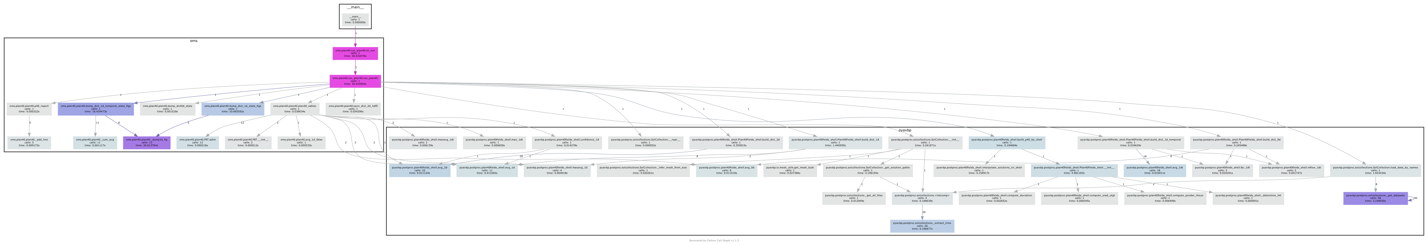
The output here is rather wide due to the structure of this specific cli_run, but this is a real-life example.
The call graph shows clearly oms, the package of the function, heavily relying on a second package pyavbp.
You can get deeper graphs by including more packages, or investigate only one portion of the graph.
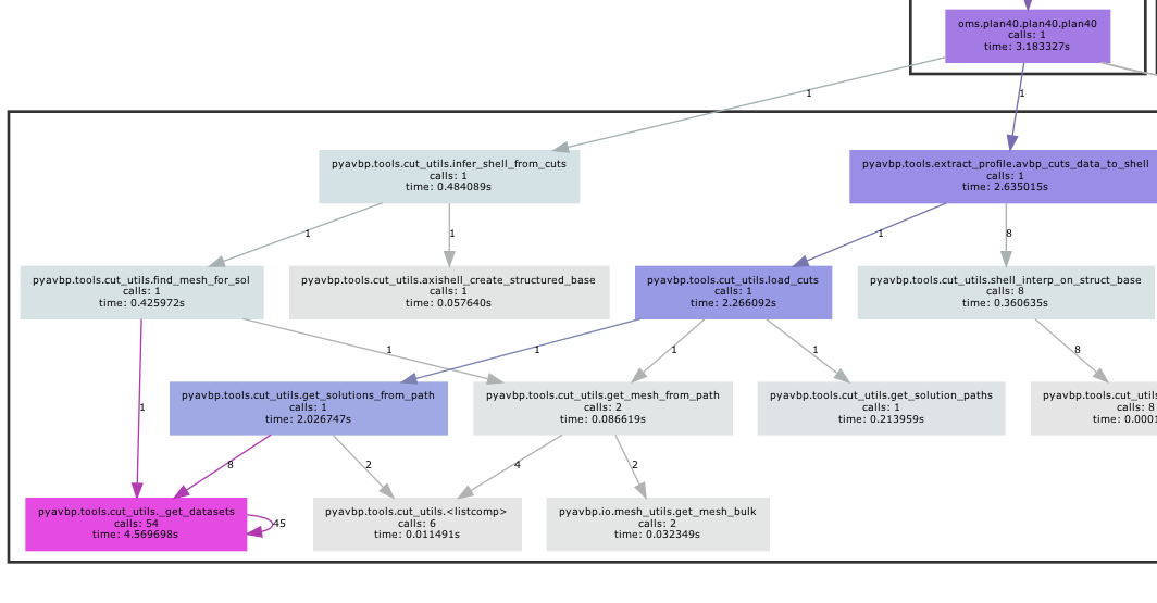
Where are the spaghetti?
The spaghetti can be visible from the call graph. The following picture focuses on an earlier version of the code. You can spot 6-8 methods are calling each other, and it is hard to figure out who called who -which is a code smell to me- . This is where we had to refactor things a lot.
So cool that I want to print it! But how?
Among the many ways to print a large image, this is a low-tech version:
- Open the image in an Excel spreadsheet
- Zoom out to see the printing zones lines
- paste your image into Excel
- resize the image to fit on the printing grid
- preview then print (BW, single page)
The static callgraph
The static callgraph generation can be done with several packages:
Before continuing, a caveat: a static callgraph is usually an approximation. You can dig deeper on this aspect in the litterature, maybe starting from this Jens Dietrich article. Simply put, when generating the graph some programming techniques of the source code -templates, strong object-oriented programming- can challenge the algorithm and yield incomplete or false graphs. For example, jonga was apparently created specifically to “handle the relatively complex class structure in the SPORCO package”, namely “method classes within a hierarchy of derived classes”.
After some painfull experiences, my personal impression is that what a static callgraph miss is often what readers find hard -if not impossible- to understand, and I rise the red flag of the technical debt.
Getting started with pycg/pyvis, generating the data
Here we will use pycg to generate the static callgraph data, then pyvis to plot it.
First install the two packages
> pip install pycg
> pip install pyvis
Then ask pycgfor your data. The following example is on my own personnal package tiny_2d_engine. Use pycg README notes to adapt the line to your case.
pycg --package tiny_2d_engine /Users/dauptain/GITLAB/tiny_2d_engine/src/tiny_2d_engine/acquisition_canvas.py -o tmp.json
The output is a brutal JSON file. The fun starts here
Plotting the output of pycg with pyvis
First we import the data into a networkX Directed graph. This intermediate load ensures a well defined graph cared by networkX, whatever the source is (Some callgraph generators can give incomplete graph definition).
import networkx as nx

def to_ntwx_json(data: dict)->  nx.DiGraph:

    nt = nx.DiGraph()

    def _ensure_key(name):
        if name not in nt:
            nt.add_node(name, size=50)
    for node in data:
        _ensure_key(node)
        for child in data[node]:
            _ensure_key(child)
            nt.add_edge(node,child)
    return nt


with open("tmp.json","r") as fin:
    cgdata = json.load(fin)


ntx = to_ntwx_json(cgdata)
print(ntx.number_of_nodes())
Once this works, we pipe it to a pyvis object:
color_filter={
    "menus": "red",
    "loader": "purple",
    "forms": "darkblue",
    "popups": "blue",
    "default": "black",

}

def ntw_pyvis(ntx:nx.DiGraph, root, size0=5, loosen=2):
    nt = Network(width="1200px",height="800px", directed=True)
    for node in ntx.nodes:
        mass = ntx.nodes[node]["size"]/(loosen*size0)
        size = size0*ntx.nodes[node]["size"]**0.5
        label = node
        color=color_filter["default"]
        for key in color_filter:
            if key in node:
                color=color_filter[key]
        kwargs= {
            "label":label,
            "mass":mass,
            "size":size,
            "color":color,
        }
        nt.add_node(node, **kwargs,)

    for link in ntx.edges:
        try:
            depth = nx.shortest_path_length(ntx, source=root, target=link[0])
            width =max(size0,size0*(12 - 4*depth))
        except:
            width=5

        nt.add_edge(link[0], link[1], width=width)

    nt.show_buttons(filter_=["physics"])
    nt.show('nodes.html')
In this function, the size node attribute will control the size of the nodes. In a more advanced version, you use here the number of statements, but let’s keep things simple for now.
The color_filter dictionnary customizes the coloring of the graph, helping the reader to instantly attribute a node to one of his/her basics mental model references.
These functions should generate a nodes.html file to open with your browser.
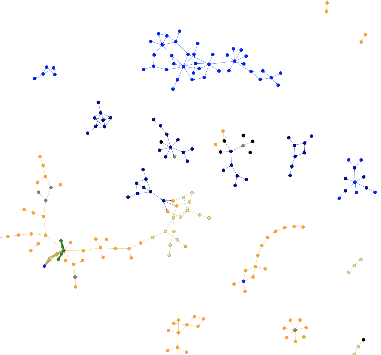
A static pycg/pyvis callgraph of a package suffering from circular import,among other problems.
Up to 100 nodes (methods or functions) , the loading is snappy. It becomes sluggish up to 2000 nodes. As the output is probably not meaningfull anymore beyond 2000 nodes, let’s filter things out!
Filtering the graph
Here are two ways to filter out your graph
We can first remove hyperconnected nodes. For example an exception handler, called by many parts of the code, like print_error_and_exit() is probably not pertinent, and will look like a “tangle point”
(...)
def remove_hyperconnect(ntx: nx.DiGraph, treshold=5):
    to_remove = []
    for node in ntx.nodes:
        if len(list(ntx.predecessors(node))) >= treshold:
            to_remove.append(node)

    for node in to_remove:
        ntx.remove_node(node)
    return ntx
(...)
ntx = remove_hyperconnect(ntx)
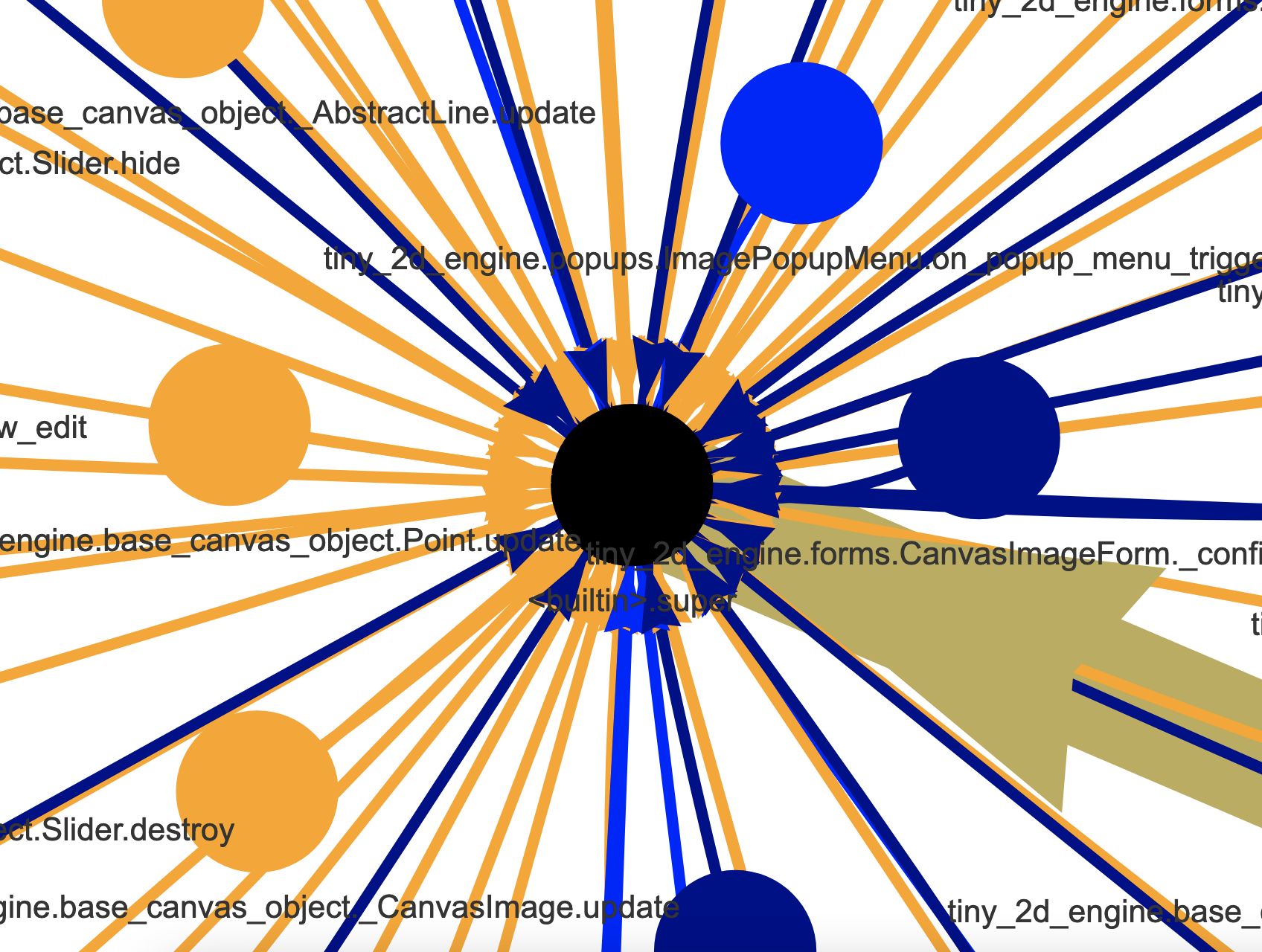
This <builtin>.super() method is at the same time hyperconnected (called by many), and from an external source. It tangle all the graph to one point, and must be removed
Then we can remove some nodes by pattern matching:
import fnmatch
(...)
def remove_by_patterns(ntx: nx.DiGraph,forbidden_names: list=[])-> nx.DiGraph:

    def is_allowed(name):
        for pattern in forbidden_names:
            if fnmatch.filter([name], pattern):
                return False
        return True

    to_remove = []
    for node in ntx.nodes:
        if not is_allowed(node):
            to_remove.append(node)

    for node in to_remove:
        ntx.remove_node(node)

    return ntx

ntx = remove_by_patterns(ntx, forbidden_names=[
     "<builtin>*",
     "numpy*",
     "tkinter*"
(...)
print(ntx.number_of_nodes())
With this, you can reduce the graph to something readable -if not enlighting-.
Practical usage
The tiny_2_engine was suffering from circular imports. Looking closer at the graph, a strange pattern is visible:
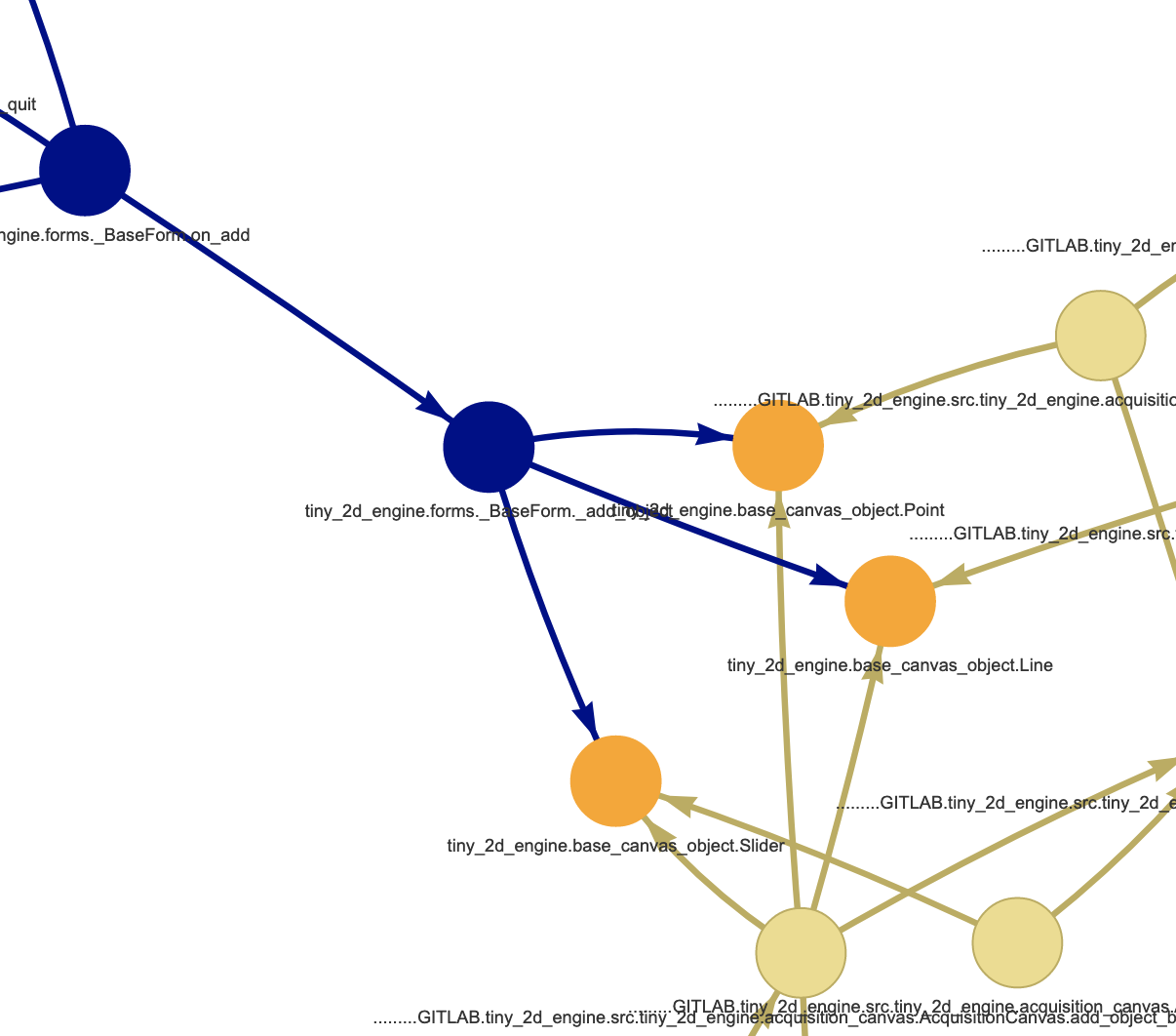
Here, three orange objects named Point, Line and Slider are called both by :
- the main
acquisition_canevas, a specializedtk.Canevas, here in Sand color - and by
forms, in blue, a topLevel form generator to create these objects on the canvas.
The solution was to limit the visibility of Point, Line and Slider to acquisition_canevas, by adding methods such as acquisition_canevas.add_line() to the main object. The forms do not need the objects anymore, and the circular import vanishes.
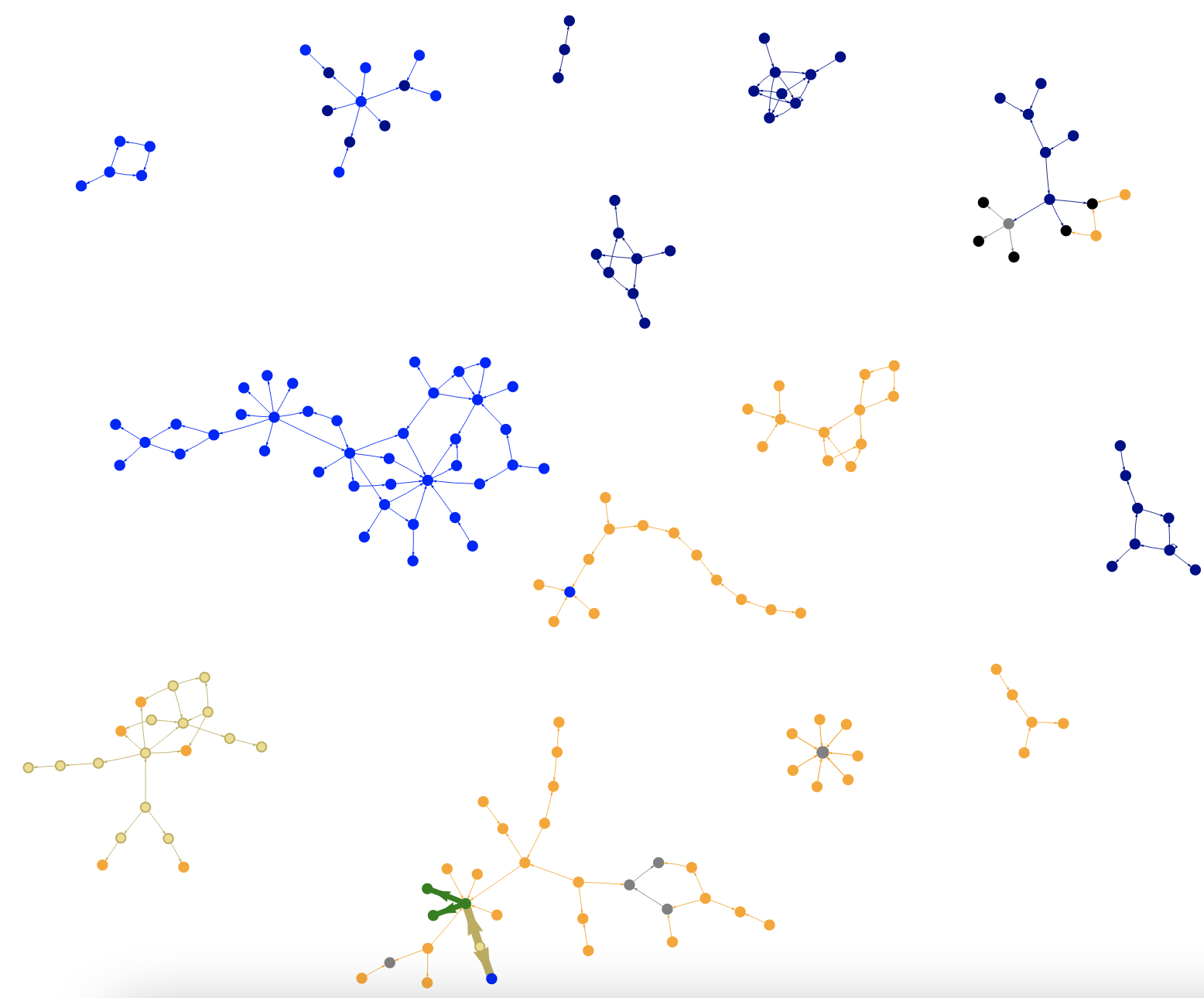
The same static callgraph without the circular import
Haem… we are not saying these now scattered graphs are an example to follow! Only that the callgraph helped to identify a solution at the method level.
Takeaway
Callgraphs are pretty useful tools - if you manage to make them understandable for your end-users. We suggest you adapt these techniques to your situation using the following steps
- Generate the call graph data.
- Prune the obvious (external dependencies) and unecessary parts(command line interfaces? deprecated content?)
- Remove the hyperconnected calls.
- If desired, limit your graph to one subgraph stemming from one node.
- Use colors to hint the source arborescence on the graph (e.g. “utils/” un grey, “core/” in red)
- Try to scale the nodes by the number of code lines
- Ask a friend for feedback on the callgraph, so you will not force your mental model on your pipeline.
We currently work on an OpenSource package able to sum this up, so you can copy/paste it to your liking. Stay tuned!
Acknowlegements
Great thanks to the many authors of these projects, especially “Gak” Gerald Kaszuba & al. (Pycallgraph), Edmund Horner & al. (Pyan), Vitalis Salis & al. (Pycg), and Pyvis team.