Anamika - A fresh approach to machine learning DSLs using visual programming

Anamika is a new Machine Learning DSL developed at ALGO-COOP based on a fresh approach to productive programming and easy hybridization of traditional differentiable HPC codes with ML models. The project derives huge inspiration from OpenModellica, which is quite evident from the name Anamika. Anamika is a Sanskrit word which has two meanings (i) a beautiful lady without a name and (ii) the ring finger (both of which are part of the logo). The hand gesture with the ring finger folded denotes the crown (or the crown chakra) the highest energy centre of the human body according to the yogic science. As an analogy we want Ananmika to be the highly productive and energetic ML DSLs out there.

You can check out a minimal working demo by clicking here -> Anamika. WASM files take some time to download, compile and execute so give it some time.

Design elements

The design of Anamika is based on the idea that one can model an arbitrary complex system using a network of simplified blocks (see figure below) whose parameters (a,b,c) can be tuned to match the behaviour of the system to inputs (in) to produce desired output (out). The source of input to this system model is shown using the block (input source). Note that several of such system model blocks can be connected to form a complex network of inputs connecting outputs. Such a model readily extends itself to represent traditional engineering systems (OpenModellica) but it is equally useful to represent Machine Learning (ML) or Neural Network models.

For ML models the system parameters translates to the weights and biases of the underlying neural network model. Therefore, such a model can be easily designed using visual elements or blocks with input/output pins which are connected using links to denote the flow of information. By combining this model with a code generation tool one can readily generate the implementation of a given model on the hardware. With the use of Algorithmic Differentiation (aka AutoDiff) tools we can obtain design sensitivities (\(sens_x\), \(sens_y\)) of the system parameters to the output perturbation (\(\overline{out}\)) thus enabling the tuning of the model to fit the input to the output (training).

Physics based constraints can be readily enforced by including blocks that represent the physical model of the system like a PDE/ODE. We show an example of such an approach in the figure below.

This makes this block-flow type visual representation quite a powerful abstraction that brings clarity and ease of use. In addition it abstracts away the implementation and programming complexity/details into the code generator. Thus, an engineer/domain expert is able to focus on designing the model for the system and tuning the parameters using his favourite optimization methods. We have currently implemented a C++ based code-generator that produces pure C code that runs on multicore CPU/GPU using OpenACC pragma. Tapenade AutoDiff tool is used to differentiate the generated sources to obtain the desired parameter sensitives to perform the training/optimization. We shall explain the code-generation and optimisations necessary to generate HPC adjoint-gradients using Tapenade in a later post.

Overview of visual elements

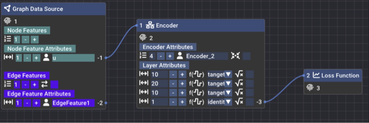
Currently, three types of blocks have been implemented to enable the design of Message-passing Graph Neural Networks, which we will explain in the following subsections.

Graph Source Block

1. Unique ID of a block (fingerprint)
2. Add node features click on the +/- buttons or directly type in input box
3. Select size of node feature (for example velocity is 3 [vx, vy, vz])
4. Input the name of node feature
5. Add edge features click on the +/- buttons or directly type in input box
6. Toggle symmetric graph edge
7. Select size of node feature (for example face normal is 3 [nx, ny, nz])
8. Input the name of edge feature
9. These are the output pins of the features for plumbing

Encoder Block

1. Input pin of this encoder block for plumbing
2. Unique ID of block (fingerprint)
3. Add MLP layer click on the +/- buttons or directly type in input box
4. Input the name of this encoder block
5. Scatter the edge encoded value to node (only applicable for mixed input features node + edge). The combo box has the {++, -+, +-} for type of accumulation - scatter to the left/right node of in the case of symmetric edge and only left node in the case of asymmetric edge
6. MLP layer settings like latent size, activation function and layer normalisation
7. Output pin of encoder for plumbing

Loss Function Block

1. Input pin of this loss function block. For every feature you like to use in the loss function connect to this input pin
2. Unique ID of block (fingerprint)

• Note that all output pins have a negative integer ID and input pins have a positive integer ID by design and every block has a unique positive integer ID that is automatically assigned by Ananmika

For a video demo of how to connect the blocks with each other and keyboard bindings please refer to the video here -> DEMO.

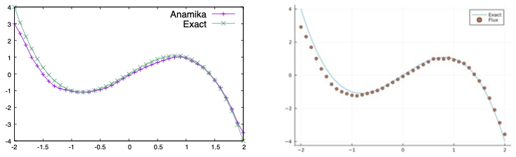
A simple ML regression model

We demonstrate Anamika on a simple problem of fitting a 4 layer MLP to approximate the function,

The Julia-Flux model and code to perform this curve fitting is shown below,

  using Flux, Plots, HDF5
  data = [([x], 2x-x^3) for x in 0:0.1f0:2];
  init_model = Flux.randn32(Flux.MersenneTwister(1));
  # init_model = Flux.kaiming_normal;
  activation_fun = tanh;
  model = Chain(Dense(1 => 10, activation_fun; bias=true, init=init_model),
                Dense(10 => 20, activation_fun; bias=true, init=init_model),
                Dense(20 => 10, activation_fun; bias=true, init=init_model),
                Dense(10 => 1, identity; bias=true, init=init_model), only);
  params_before = deepcopy(Flux.params(model));
  optim = Flux.setup(AdaGrad(), model);
  for epoch in 1:500
    Flux.train!((m,x,y) -> (m(x) - y)^2, model, data, optim);
  end

  plot(x -> 2x-x^3, 0, 2, legend=false)
  scatter!(0:0.1:2, [model([x]) for x in 0:0.1:2])

Using the model generated from Anamika DSL we supply the random initialised parameters from Julia to verify if we can reproduce the same results as Julia. It is possible to write the parameters of the Julia to a HDF5 and the same ordering is enforce in Anamika. The code to generate the HDF5 parameter file is show below,

  flat_params = Vector{Float32}()
  for item in Flux.params(model)
    append!(flat_params, collect(Iterators.flatten(item)))
  end
  print("Total number of params = ", size(flat_params)[1])
  fid = h5open("params.h5", "w")
  fid["params"] = flat_params
  close(fid)

We find that the model evaluation exactly matches the Julia-Flux model and the Anamika generated C code as shown below.

The test code to run the model is given below,

#include <iostream>
#include <hdf5.h>
#include <vector>
#include <sstream>
#include <fstream>

template <typename T>
static int read_hdf5_data(hid_t &file, const char *link, hid_t &dtype, T *buf) {
  if (H5Lexists(file, link, H5P_DEFAULT) == 0) {
    std::stringstream cat;
    cat << "Error: Cannot find dataset " << link << " in hdf5 file";
    throw std::runtime_error(cat.str().c_str());
  }
  hsize_t dims[10];
  hid_t dset = H5Dopen(file, link, H5P_DEFAULT);
  hid_t dspace = H5Dget_space(dset);
  int rank = H5Sget_simple_extent_dims(dspace, dims, NULL);
  herr_t status =
      H5Dread(dset, dtype, H5P_DEFAULT, H5P_DEFAULT, H5P_DEFAULT, buf);
  assert(status >= 0);
  H5Sclose(dspace);
  H5Dclose(dset);
  return rank;
}

extern "C" {
  void run_network(const int nnodes, const int nedges, int *edgelist, float *params, float *EdgeFeature1, float *u, float *xout3);
};

int nnodes = 41;
int nedges = 1;
int nparams = 305;

std::vector<float> params(nparams);
std::vector<float> EdgeFeature1(nedges);
std::vector<float> u(nnodes);
std::vector<float> xout3(nnodes);
std::vector<float> xout3_ref(nnodes);
std::vector<int> edgelist(nedges * 2);

int main(int nargs, char *args[]) {
  // Init the values
  // data = [([x], 2x-x^3) for x in -2:0.1f0:2]
  for(int i=0; i < nnodes; ++i) {
    const double x = -2.0 + i * 0.1;
    u[i] = x;
    xout3_ref[i] = (2.0 - x * x ) * x;
  }
  // Read params from HDF5 file
  auto file = H5Fopen(args[1], H5F_ACC_RDWR, H5P_DEFAULT);
  read_hdf5_data(file, "params", H5T_NATIVE_FLOAT, params.data());
  run_network(nnodes, nedges, edgelist.data(), params.data(), EdgeFeature1.data(), u.data(), xout3.data());
  H5Fclose(file);
  std::ofstream fout("plot.dat");
  for(int i=0; i < nnodes; ++i)
    fout << u[i] << " " << xout3[i] << " " << xout3_ref[i] << "\n";
  return 0;
}

On going work

We are currently working on an automated workflow for code-generation, AutoDiff and training using a scripting language based on Scheme lisp Guile. This will give the user to tinker with the complete worflow which are generated and given to them in the form of Guile Scheme scripts.

We are also working on a lisp DSL to represent the visual blocks and connections so that users will have the option to write lisp scripts to auto-generate network code and train them. This will be extremely useful for exploring various network architecture and activations functions, optimal layer size selection in an automated fashion.

Open Graph Drawing Framework (OGDF) is being leveraged to create better layout and visualisations when the size of the network increases. We will also replace our hand rolled graph algorithms like topological sort and depth first search with the ones from OGDF.

Acknowledgement

We like to thank @ocornut for his Dear-Imgui library, @Nelarius for his imnodes library, @BalazsJako for his ImGuiColorTextEdit library. The online demo was made possible by the Emscripten compiler that compiled the C++ sources of Anamika to WASM (web assembly). Finally the SDL2 library was used for window and keyboard/mouse control and OpenGL3 for the graphics rendering.

Like this post? Share on: Twitter ❄ Facebook ❄ Email