TDL - Tékigô Deep Learning
TDL is a tool to predict the node-number of a mesh after a mesh-adaptation by MMG library.
Background - CFD and numerical mesh
CFD (Computational Fluid Dynamics) is a numerical study to simulate the behavior of a fluid such as air flow in an aircraft engine. In CFD, we describe a continous domain by scattered points as in the right in Fig.1. This is called discretization and the discretization domain is called “mesh”. The distribution of mesh points, also called “nodes”, largely affect the quality of the accuracy of simulation. MMG library is a tool to re-distribut the points to increase accuray. Fig.1 shows an example of an adaptation to a temperature field in the left of the figure.
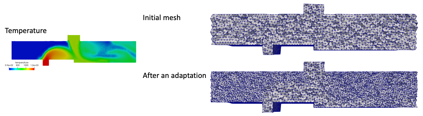 Fig.1 Example of numerical mesh and its adaptation to a temperature field
Tékigô
What it does
Our mesh-adaptation tool Tékigô performs a mesh adaptation by a system based on MMG library. The difference from MMG library is that Tékigô can specify the target node-number after the adaptation and can mix up multiple conditions (ex. concentrate points on a lower temperature and high velocity zone).
Metric
In Tékigô, a variable called metric is defined at each node. This variable basically means how much you will increase the mesh at each node (ex. when metric = 2.0 is given on a node, this node will be devided into two nodes). Fig.4b is an example of metric. Here metric is set to refine the mesh outside of a flame (metric < 1.0) and coarsen the inside (metric > 1.0). MMG library integrated in Tékigô reads metric as input and refines the mesh.
Modification of metric by node-number estimation
MMG library can only specify metric and is unable to specify the node-number in advance of the adaptation. To make it possible, Tékigô has a “trial and error” process as shown in Fig.2. It estimates the node-number based on the metric at first. If it’s far from the target, metric will be modified so that the node-number gets closer to the target. When the estimated number is enough close to the target, Tékigô finally runs an adaptation by MMG library.
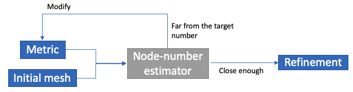 Fig.2 “Trial and error” process in Tékigô
TDL improves the node-number estimation
The problem is that this estimator can have around upto 20% of error. TDL was developed to give a better estimation of the node-number of a mesh. It has an integrated UNet-type Deep Learning inside (described below). The network inside is pre-trained with various case of adaptations. In the current version, the error of the node-number estimation is reduced to 2-5%. A better estimation of the node-number will reduce the iterative “trial and error” process of the modification of metric. This will allow Tékigô to generate a better mesh with less execution time.
How it works
In TDL, a new node-density field is predicted from metric and the “node-density” calculated by the initial mesh. Then the node-number will be calculated by the integral of this node-density. Fig.3 shows how those things work inside. Its algorithm will be explained in detail below.
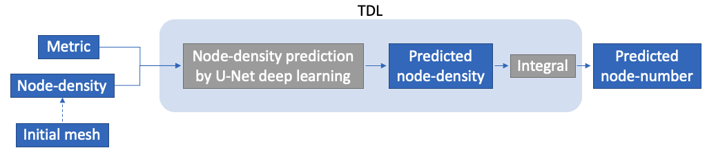 Fig.3 How TDL works to estimate node-number
Algorithme
1. Calculate the node-density
We consider a variable called “node-density”. This is calculated by the inverse of the cell volume (cell-surface area, if 2D). The dimension of this variable is [number of nodes / unit volume or surface].
2. Interpolate to a Cartesian grid
The cell volume is defined at the center of gravity of a cell. To perform UNet-type Deep Learning, a rectangular image where each dots are distributed like a Cartesian-grid is needed. So the cell volume field will be interpolated to a rectangular grid. This is done by a simple command of Python griddata((xcell, ycell), dens_node, (X, Y), method='cubic') where (xcell, ycell) are x,y-coordinates of cells and dens_node is node-density field, (X, Y) are the coordinates of Cartesian-grid on which we interpolate. method='cubic' means the cubic method for the interplotion. Fig.4a shows the node-density field interpolated to a Cartesian-grid-like image. Here we take an example of an adaptation on a mesh the cell volume of which is uniform everywhere in its whole domain.
3. Prediction of the new node-density field
UNet-type Deep Learning reads the metric and the node-density as input and outputs a new node-density field which is expected to be formed after this adaptation with this metric and the initial node-density. Let’s consider a metric field like Fig.4a and the node-density field of Fig.4b as the input. By the prediction of Deep Learning, we gets a new node-density field like Fig.5a. Just for comparison, the image on the right Fig.5b is the image after the adaptation. The node number will be estimated by this predicted node-density (see next step). Obviously the reproductivity of the image Fig.5a compared to the real image Fig.5b is linked to the precision.
4. Estimate the node number by the adaptation
Calculate the integral of the predicted node-density field (Fig.5a-left). This gives the total number of the nodes.
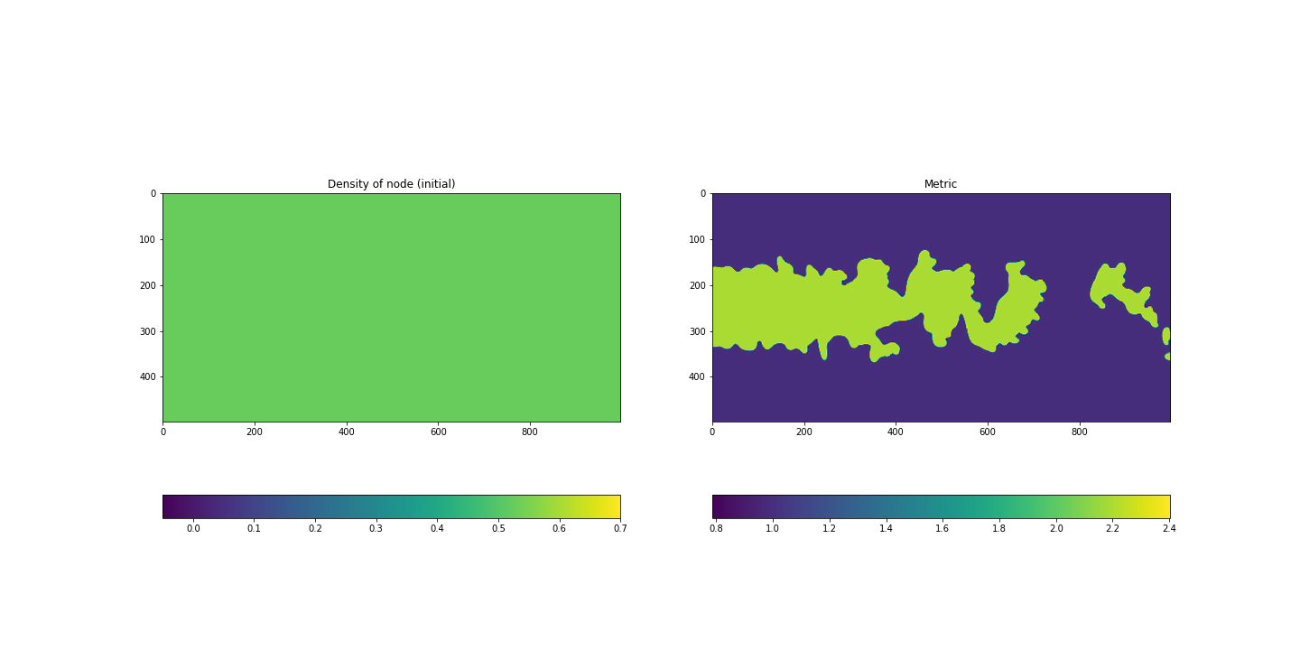 Fig.4a Node-density before an adaptation(left), b Metric(right)
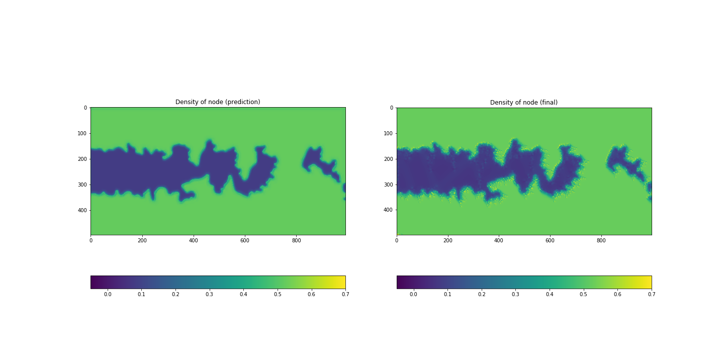 Fig.5a Predicted node-density(left), b Node-density after an adaptation(right)
Neural network for the prediction
Fig.6 shows the configuration of the implemented network. This type of network is called UNet, which was named after its U-like shape of encoder-decoder network for semantic segmentation (see also A Beginner’s Guide to Neural Networks and Deep Learning). It was originally designed for biomedical image segmentation. The network used in this tool has only two layers for each side (encoder-decoder). The size of the images for the input varies depending on the case. To handle this, a section of 256x256 is truncated from the original images and used as the input images. The location of this section is randomly chosen in the domain.
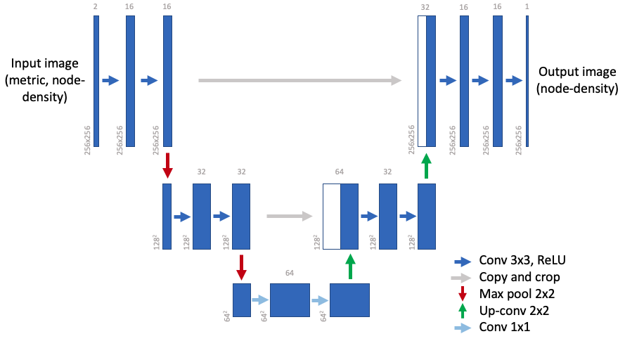
Fig.6 Neural network for the prediction
Use case
Although a wide variety of mesh-adaptation of different kinds of simulation would be an ideal data-set to train the neural network, it doesn’t seem realistic to collect the data-set by such way. In stead, we used a fire-flame simulation and generated a few hundreds of meshes which are different from each other. A simulation of droplet-evapolation is also used to generate a data-set in order to diversify the data-set for the test.
1. Data generation
Those simulations are time variant (= unsteady), which means that the shapes of the flame and the droplet-evapolation vary in time. The mesh is constant but the simulation result changes every step of simulation. Now if we run an adaptation of Tékigô on a set of simulation results and the mesh of each instant, we would get a data-set of which each elements differs in theory.
Let’s just look at how we generated the data-sets to understand this. Fig.7 shows the strategy to generate the data-sets. For example, the flame case for the training and the validation were generated from 6 different instants of the simulation. On every one of 6 instants, the adaptation was done on 3 variables and 4 target-numbers with 4 steps to get to the target (the adaptation generates a mesh at each step of the loop, see Fig.4 in our blog of Tékigô for this inner loop). The initial mesh is of 131841 nodes. Finally this makes 6 x 3 x 4 x 4 = 288 cases of adaptation. Data-sets for the two tests were done by such process.
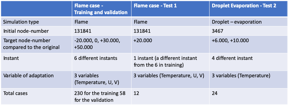 Fig.7 Mesh generation strategies
Fig.8 shows the overview of the data for the training, the validation and the test
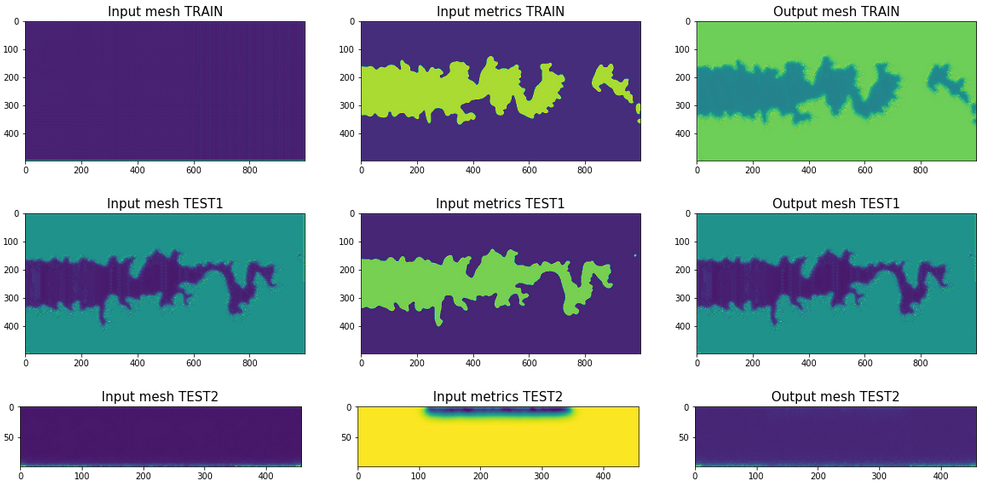 Fig.8 Overview of the data for the training, the validation and the test
2. Learning by neural network
We use exactly the same UNet-type neural network as described in Fig.6, and train them on the data-set generated in the previous step. The data augmentation based on partial extraction was used. This allows to truncate a part of a whole original image. By this we get multiple (but in truncated size) images from the original images.
Fig.4 and Fig.5 shown previously are an example of prediction on a flame case. With the node-density of the inital mesh in the Fig.4a and the metric-field in Fig.4b, our neural network gives back a prediction of node-density after the refinement as in Fig.5a, which correponds well to the real node-density after the refinement. The same figures on before/after the refinement of test2 are shown in Fig.9 and 10. It’s a bit hard to judge the prediction worked well.
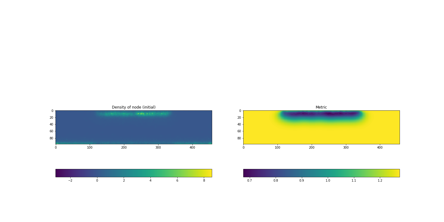 Fig.9a Node-density before an adaptation(left), b Metric(right) of test2
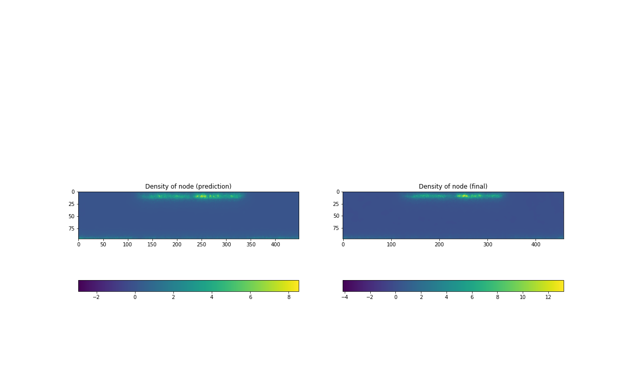 Fig.10a Predicted node-density(left), b Node-density after an adaptation(right) of test2
A comparison on the node-number calculated from the images give us a clearer view on the performance of our prediction. The following table shows the errors of the preditions by our newral network to the real node-numbers of refined meshes. In a general sense, our neural network TDL give largely better results on all the types of data-set.
| Estimator in Tékigô | TDL | |
|---|---|---|
| Training data | 7.5182% | 2.3877% |
| Test1 | 13.343% | 3.6973% |
| Test2 | 44.323% | 24.151% |
3. Source code
For futher details, see the source code.