Reading time: 18 min
This work is part of COEC-WP5 is a center of excellence dedicated to simulation software that can support the decarbonization goals and run on Exascale supercomputers.
It introduces a CFD mesh generation procedure trought recursive mesh adaptation. A demonstration is given for the mock up trapped vortex burner geometry simulated with CERFACS AVBP CFD flow solver, followed by an application to an European-level academic configuration for combustion, the PRECCINSTA burner.
Motivation
A CFD simulation is as good as its mesh definition.
Whichever the CFD turbulent description approach one adopts, be it RANS, LES or DNS, the results you can obtain will heavily depend on the selected mesh. Countless man hours are spent creating the “best” mesh or devising refinement strategies which will hopefully give you a result which will run on the available computational resources.
The art of meshing is heavily experience related. We know that near a shock wave more cells need to be introduced in order to not diffuse the shock over too many cells. We know that far away from a body of interest, where not much physics occur, we do not need as many cells as near the body (see e.g. Spalart, PR., and Streett, C. Young-person’s guide to detached-eddy simulation grids. NASA Langley, 2001.). We know that a certain number of cells would be required in a boundary layer and we know approximately the time step sizes that can be expected in our problem based on prior experience with the same CFD solver in similar settings. We do also have an idea of what number of grid points (or cells) are required in a certain setup to give us results within a degree of confidence.
Can we express this experience as elements of an automated meshing workflow? Can we move from an indirect best practice like “use 0.08 mm cells here to get the proper flame resolution” to a direct expression like “use 4 cells in the flame width”?
Illustration on the mock up TrappedVortex
The TrappedVortex is a lightweight configuration to test CFD tools. While simple, it features the typical complexities of combustion devices: a jet in crossflow, a recess, a film and an axi-periodic frontier. All informations, including ways to get the mesh, are available on this resource: trapped vortex.
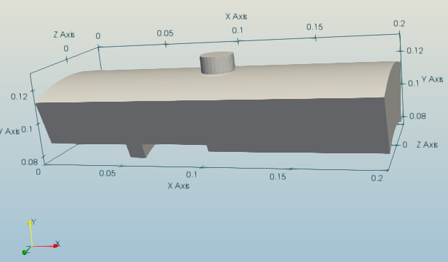
We will consider AIR (single species) as the working fluid which is injected through two inlets: the left inflow boundary (Inlet) and the top hole boundary (InletHole). Respective mass flow rates are set to 0.1 and 0.01 kg/s. Ambient conditions are selected at T = 300 K and p = 1013 hPa. All physical walls are treated as no-slip adiabatic boundaries. A non-reflective outflow is prescribed with a target back pressure of 1000 hPa.
The baseline coarse grid is described in Setting up AVBP runs and consist of 177 563 tetrahedral elements with 34 684 nodes. The simulation is run with LES and the Wall Adapting Local Eddy-viscosity approach (WALE). The CFL is set to 0.7 for a 2nd order Lax-Wendroff scheme. An initial simulation is run for 6 flow-through-times to get rid of any initial transients. The strategy described below starts from the resulting end point of the above simulation.
The automated mesh generation workflow
This mesh generation procedure is, at the end of the day, a sequence of many runs on the cluster. The procedure is the following
- Run the CFD solver to simulate a used-defined characteristic time
- perform a mesh adaptation on the latest CFD results.
- interpolate the latest solution on the new mesh
- loop
A typical workflow is illustrated in the following figure. In the present case, mesh refinement create bigger meshes. As meshes get finer, more and more jobs on the cluster are needed to simulate the same characteristic time.
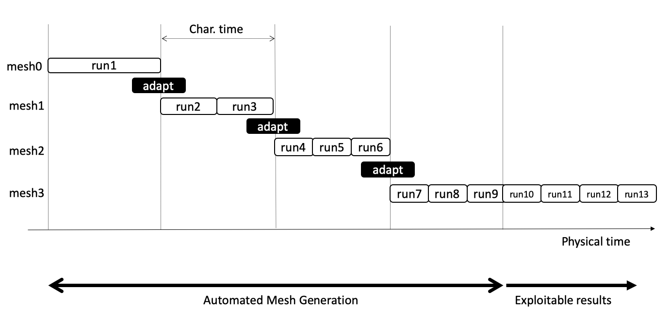
This sketch illustrates that the number of runs is unknown in advance. The job submission procedure must adapt the job nature (and duration) to the the situation.
The process can be done manually. To automated of the whole procedure, we used the open-source Lemmings workflow runner, developed in the CoE Excellerat.
The mesh adaptation step
We use here Tekigo, an open-source python wrapper suited for static unstructured mesh adaptation through HIP and MMG. See the regularly updated introductory page for more informations. Tekigo has two main approaches: raw adapt and refine, In brief,
- The raw adapt functionality takes as input a single metric field and performs a one-time refinement. The metric field is a direct representation of the desired target edge length with respect to the current one.
- The refine functionality takes in as argument multiple criteria, with each criteria ranging between -1 and 1 and representing a desired outcome (0: no refinement, -1: max coarsening, 1: max refinement). The criteria, provided as functions, are blended together by Tekigo which creates a single metric field.
The refine functionality works with additional user-defined inputs such as, target minimal edge size, target number of nodes.
An illustration of the refine function for our present aim would be
refine(tekigo_sol,
        custom_criteria,
        dry_run= False,
        nnode_max = nnodes_tgt,
        min_edge = min_edge_tgt,
        iteration_max = 1,
        met_mix = 'average',
        coarsen=False)
Where we have:
- tekigo_sol: the current flow field solution (as a Tekigo object) containing the information used in the refinement
- custom_criteria: a dictionary containing the different criteria functions to be used
- dry_run= False: deactivation of dry_run mode, we want to perform the adaptation
- nnode_max: a limit on the maximum number of nodes that we wich to have (set to “nnodes_tgt”)
- min_edge: the minimum edge size that we wich to have (set to “min_edge_tgt”)
- iteration_max: maximum number of recursive iterations to perform. We will only consider 1 iteration throughout this example
- met_mix: how to combine the criteria from custom_criteria. We consider an average of the different fields.
- coarsen=False: in our present example we will avoid coarsening and only refine the mesh in the different adaptations.
The refinement strategy
We will now complete the information required by the refine function introduced above.
custom_criteria
Our first Quantity of Interest (QOI) is the Loss In Kinetic Energy (LIKE) and is described in Daviller, G. et al. “A mesh adaptation strategy to predict pressure losses in les of swirled flows.” Flow, Turbulence and Combustion 99.1 (2017): 93-118.
The presence of walls hint at another important QOI: the y+.
Both, the LIKE and y+ are therefore considered in this example as time averaged quantities.
For the demonstration, we use here binary criteria:
- A value of 1 is set to the nodes where LIKE > 1e4.
- A value of 1 is set to the wall nodes where y+ > 20. This field is “dilated” two times over the connectivity, flagging two layers of cells near the wall.
The LIKE criterion threshold is based on the visual representation depicted in Fig. 2 which shows that, for the centerline cut, it covers regions where the jet is active as well as separations near the cavity and the step. It has minimal overlap with the y+ based criterion.

In this example we would like to have y+ values at a maximum of 20 to apply wall functions. In addition, two passes of the “dilate” feature (see also this post) are employed as to propagate the criterion, which is only defined at the wall, to the neighboring cells.
met_mix
The criteria based on LIKE and y+ are combined to form a single criterion which is the average of both: met_mix = 'average'. A subsequent conversion from a criterion (usually ranging from -1 to 1) to a metric (ranging between 0.4 and 4) is performed by Tekigo.
Because we used very simple criteria and mixing, the metric is either:
- 1 where no criteria was triggered.
- 0.7 where one of the criteria was triggered.
- 0.4 where both criteria were triggered.
However in a normal adaptation, it would be preferable to use a LIKE criteria proportional to a LIKE field filtered from its outliers, a smoother y+ mask, and probably a local minimum mixing to create the metric.
nnode_max In our present example we wish to have a resulting grid which does not exceed 300 000 nodes (= nnodes_tgt) which is approximately 1.5M tetrahedral cells in this setup.
min_edge The minimal edge size may restrict the global time step in an explicit time-stepping scheme. Therefore, an additional restriction has been introduced : a minimal edge size (min_edge_tgt) is specified based on the solution and a minimal allowed time step. Presently, we wish to have a minimum time step of 1e-7 s = dt_min_tgt.
The procedure is as follow:
- The minimal time step of the latest instantaneous solution is found: dt_min
- The node where the minimum is observed is identified:
- The edge lengths are estimated based on the volume associated with each node and assuming isotropic cells:
approx_edge_from_vol_nodefunction within Tekigo. - The edge length associated to the node where the minimal time step occurs is retrieved: edge_dtmin
- min_edge_tgt is computed as
edge_dtmin / (dt_min / dt_min_tgt)
The simulations are allowed to run for one flow through time providing the averaged fields. The refinement is then performed ,and the simulation is resumed from the new mesh and latest instantaneous solution interpolated on it. The process is then repeated for a number of times.
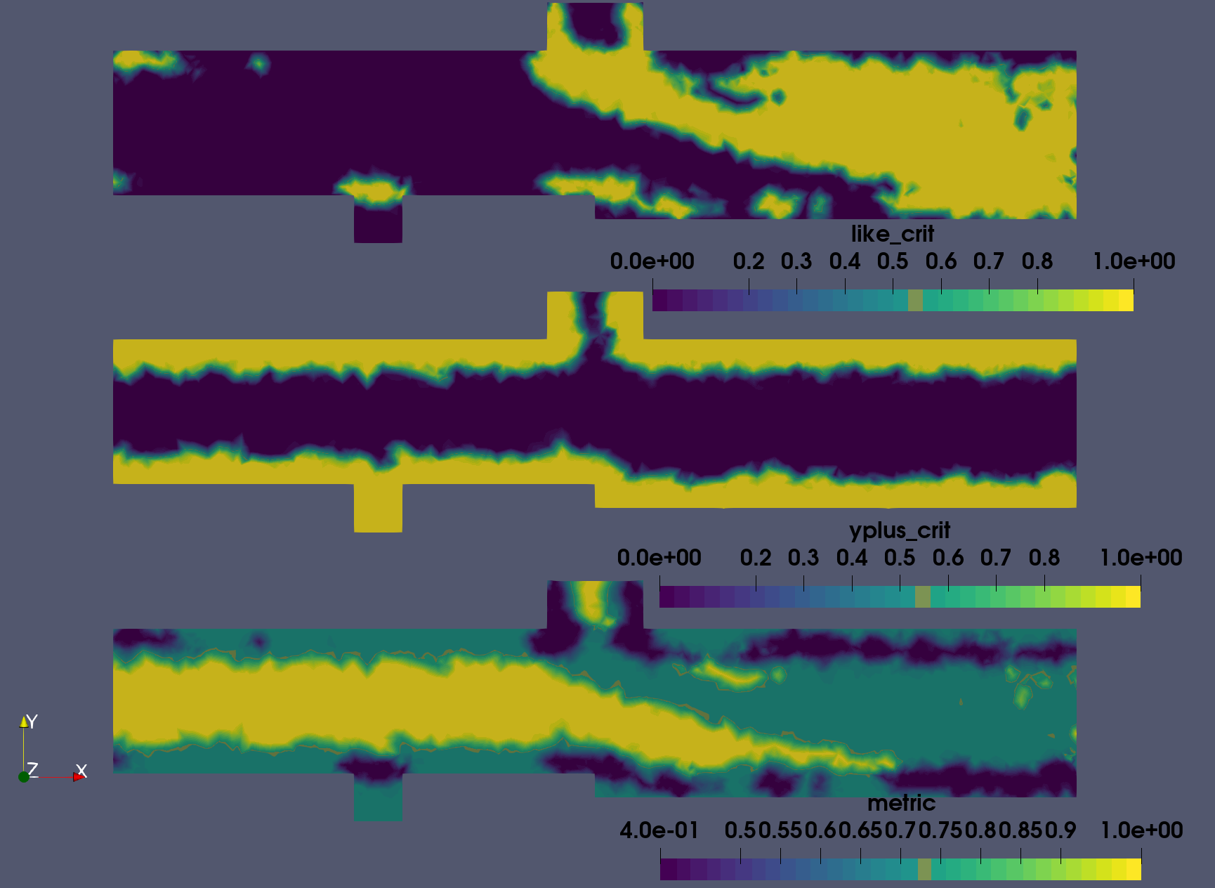
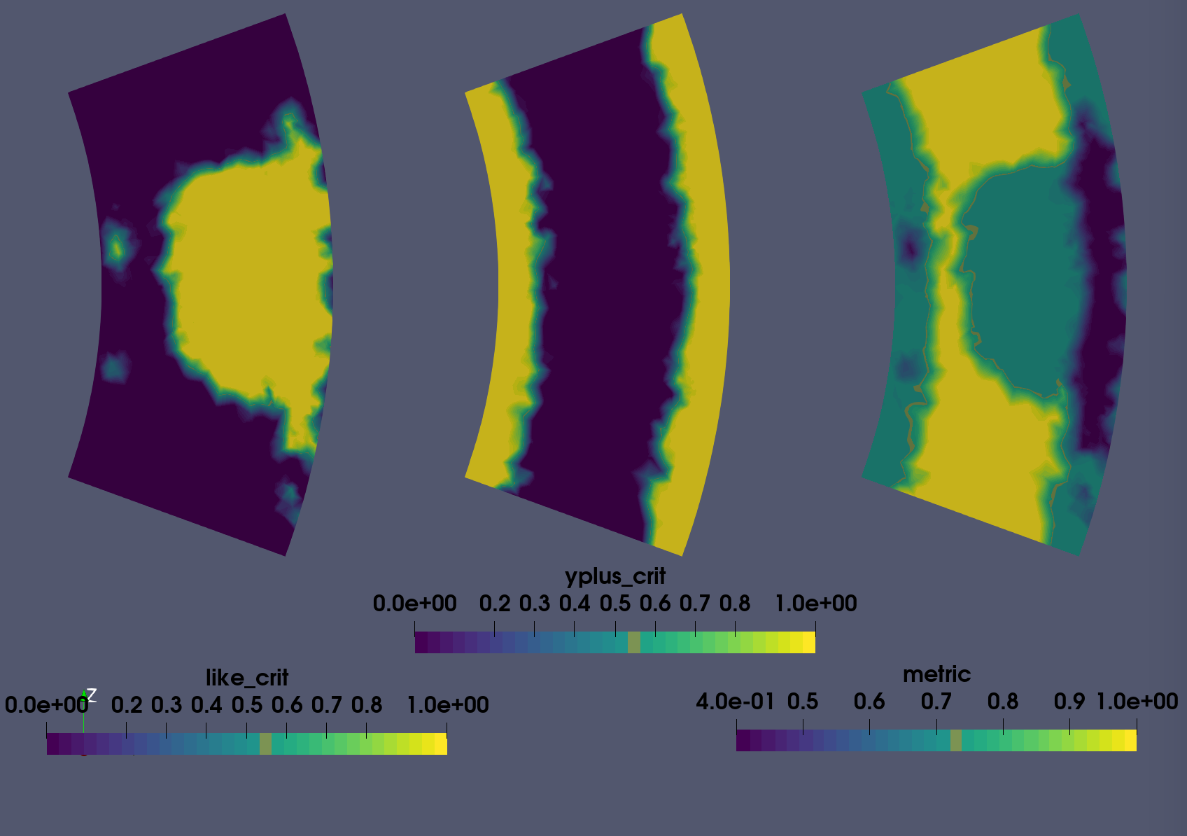
The criteria and metric
Fig 3 presents these fields for the first refinement. In accordance with Fig. 2, the LIKE criterion covers regions of flow separation and the unsteady jet. The y+ criterion, mostly covers other areas within the geometry which shows the good combination of both quantities. This is reflected in the metric field, with only some regions near the wall where both criteria are active. A cut at a stream-wise location downstream the upper injector is presented by Fig.4. It shows the jet centerline and confirms that the refinement will affect the jet region.
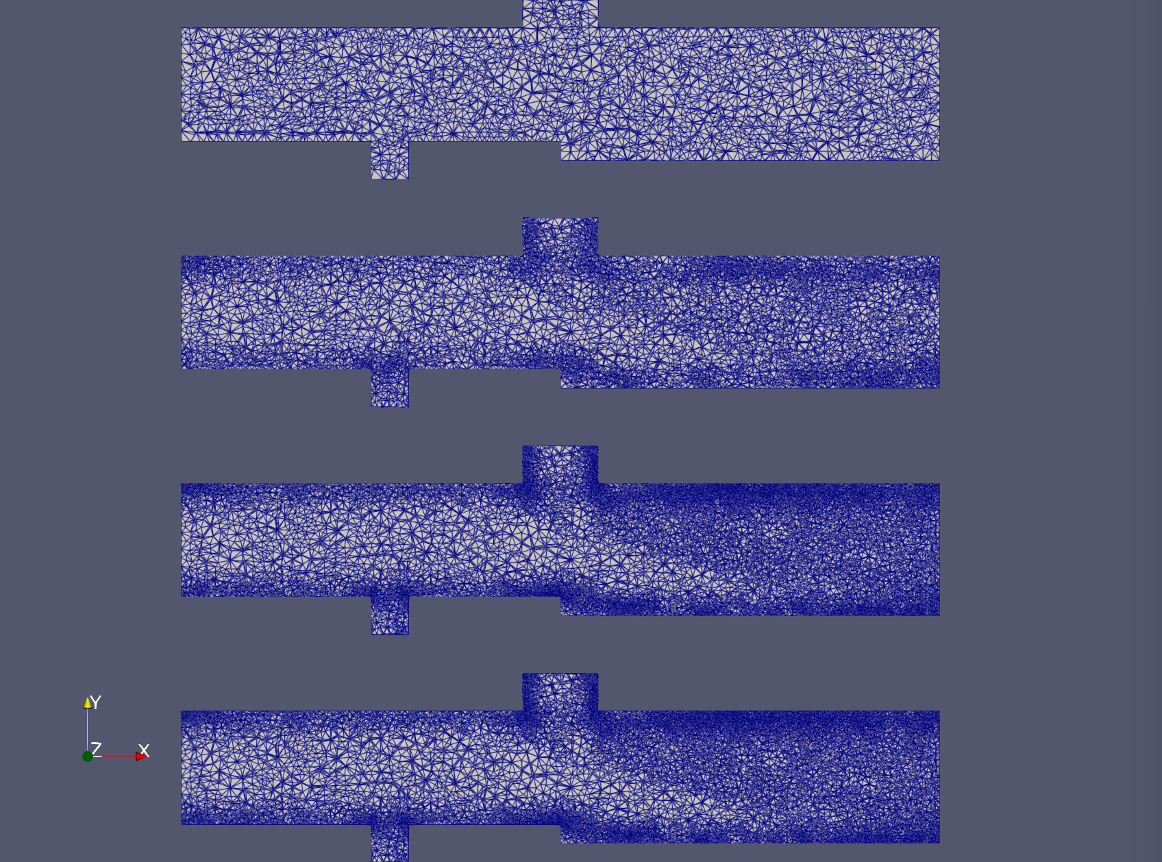
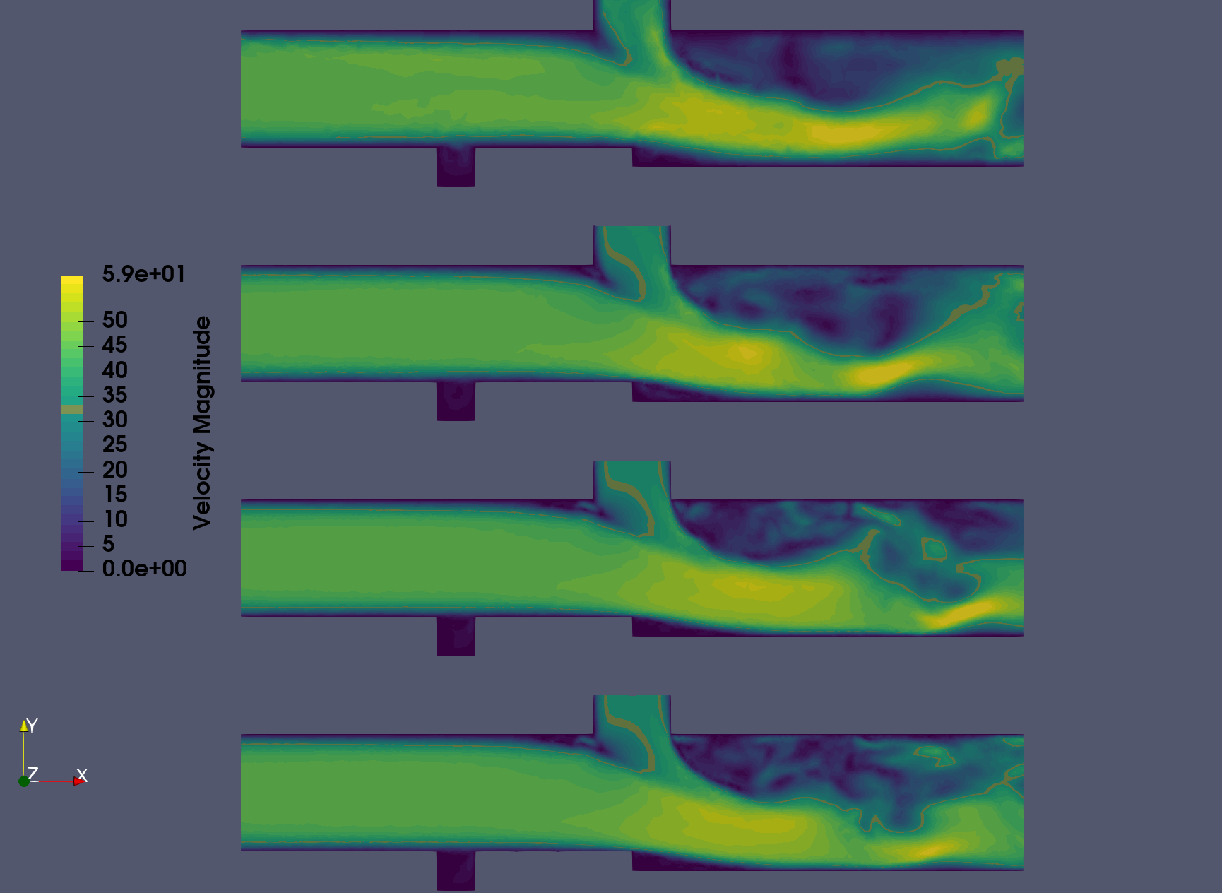
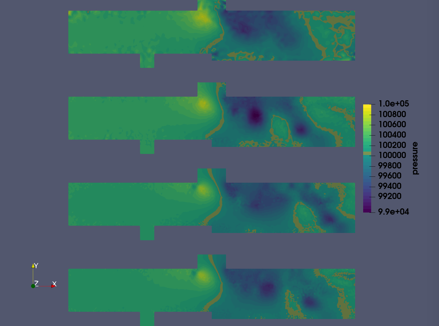
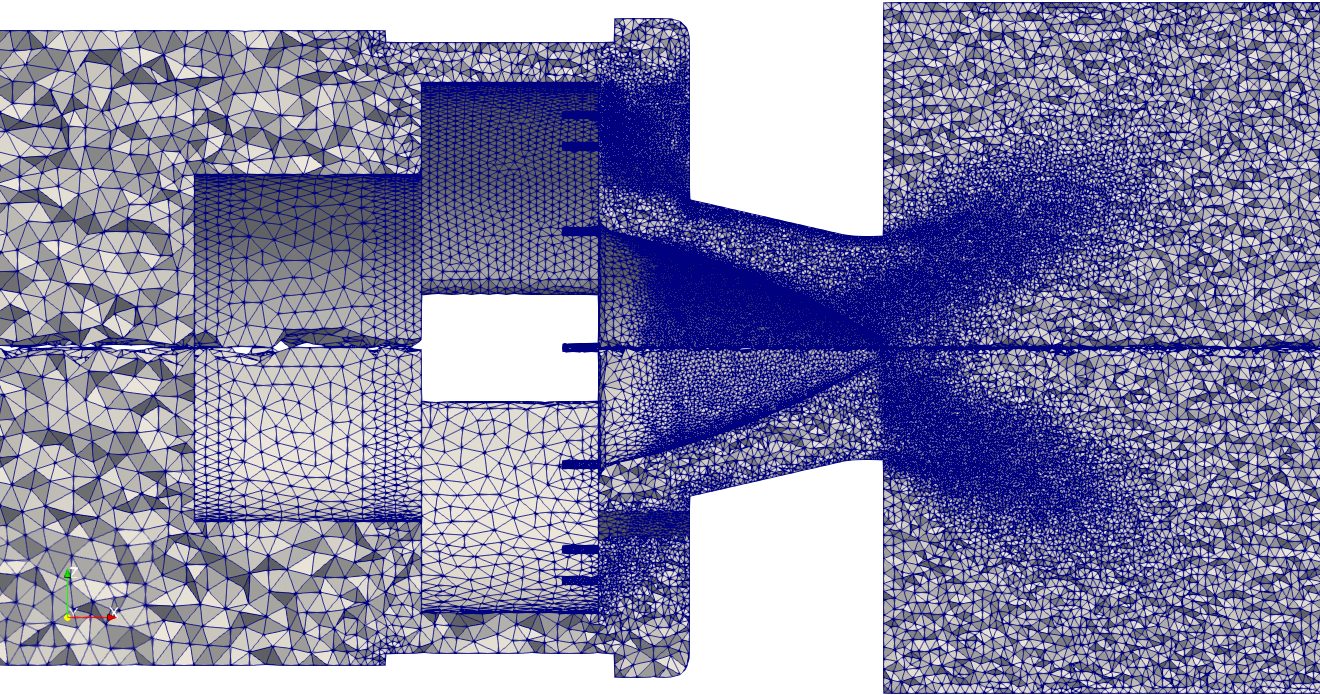
The refinement
Results of the first few refinements are given in Figures 5 to 7. The baseline grid and fields are as well presented. The refinement is mainly impacting the upper injector region with the jet’s wake and the backward facing step. As the process evolves, the upper wall downstream the upper injector is more impacted which is in line with the metric field depicted in Fig.4. It goes hand in hand with the increased resolution near the jet which result in the capture of more turbulent structure and the unsteady dynamics of the jet. The latter is shown in Fig 6. Other near-wall regions are less strongly impacted during the refinement.
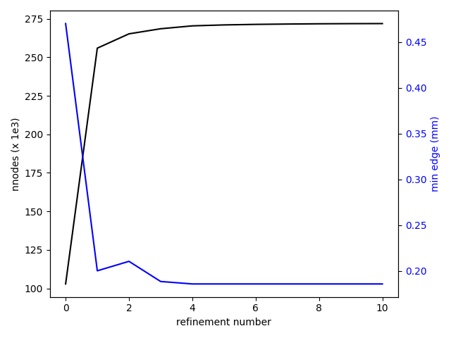
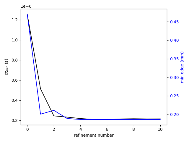
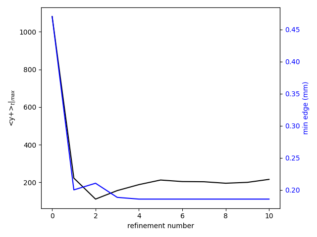
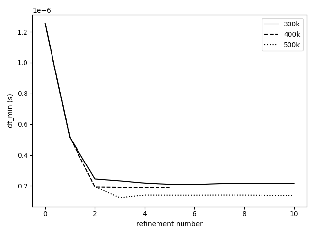
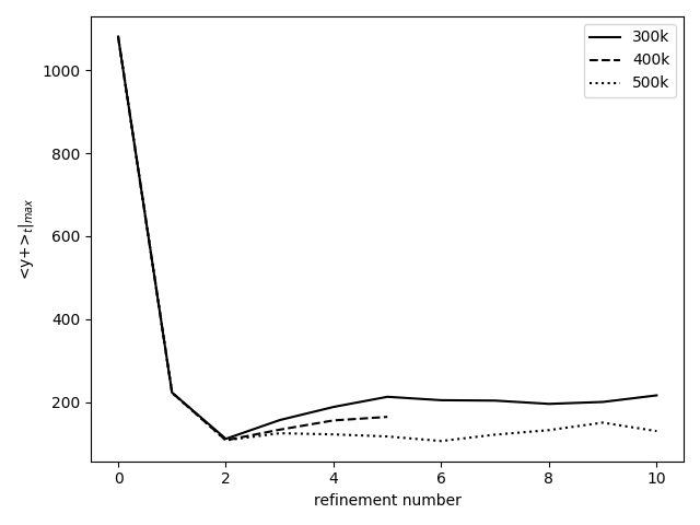
The complete workflow has been run for 10 refinement steps. Looking at Figures 8 to 10, there is a converging behavior in the static refinement. After the 4th refinement, the increment in node number becomes very small (Fig.8) and a plateau ~ 270 000 nodes is reached. It is coupled to a convergence in allowed minimal edge size which is presently coupled to the minimum desired time step. The last variable stagnates around 2e-7 s , close to the target of 1 e-7 s and the minimal edge size remains around 0.19 mm (Fig.9). The converging behavior has implications on the maximum time averaged y+ which starts well above 1000 and remains around 200 after the 5th refinement. While our desire was to obtain y+ values below 20, the imposed constraints do not allow for such levels to be reached.
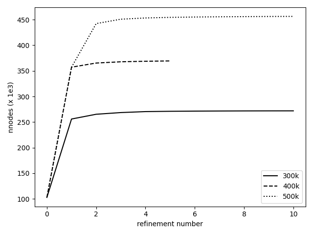
To ensure the repeatability, additional simulations have been run with maximum targeted node numbers of 400 000 and 500 000. The results are presented in Figures 11 to 13. In all cases a converging behavior is observed. The larger the target maximum node number, the closer the time step to the minimum allowed value of 1e-7 s (Fig.12). The maximum time averaged y+ (Fig.13) shows that the first few refinements impact this value in a similar manner, regardless of the target node number. Thereafter, a lower maximum value is obtained with a finer grid.
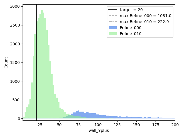
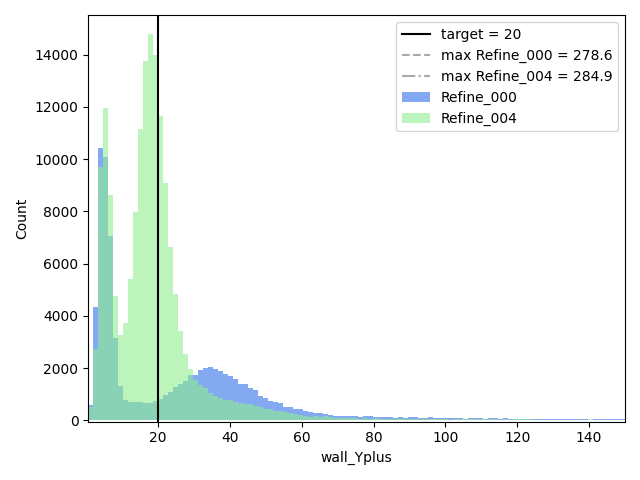
In terms of the evolution of the criteria-related quantities, the distribution of y+ and LIKE are presented in Figures 14 and 15, for the case with target maximum node number of 300 000. The y+ related criterion targeted the nodes with a mean value above 20. Fig.14 shows the progress in the distribution between the original mesh and the latest refinement. For clarity the visible portion of the x-axis range has been limited. The majority of the y+ values are reducing but they mainly remain above the target of 20.
In terms of LIKE, the refinement does show the increasing behavior with many more cells being affected by the criterion.

Comparing this workflow with present meshing practices
Now this mesh generation workflow is working, how does it compare with present meshing practices on a Combustion chamber?
In this task, we use one of the most recent simulations of the PRECCINSTA Burner, from Static mesh adaptation for reliable large eddy simulation of turbulent reacting flows Agostinelli et al. Physics of Fluids 33, 035141 (2021). The 10 million cells mesh of the paper is used here as the reference case 0.
Note that the mesh adaptation used in the article is a manual succession of direct static mesh adaptations, where the mesh size (10 million Cells) is an output of the adaptation process. Moreover, the two criteria used are applied consecutively. On the contrary in the present workflow, several non-dimensional criteria are influencing the metric simultaneously : Y+, LIKE, Minimal timestep, in an automatic recursive loop converging to a user-defined mesh size of 10 million cells.
The three simulations
All simulations are run using the same operating points, numerical setup and computational resources, with the same version of the Large Eddy Simulations software AVBP.
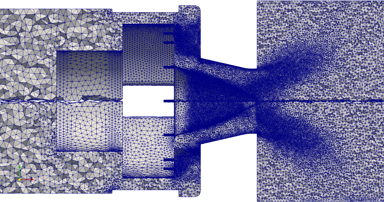
The mesh of the reference simulation 0 was manually coarsened in the swirler where there is no combustion. The perturbed case 1 is using only 6.5 Million cells.
Finally, we used the automatic mesh workflow to build, from the perturbed mesh 1, a new mesh equivalent to mesh 2. This repaired case 2 is about 9.5 million cells.
| Case | cells nb. (106) | Time step [s] |
|---|---|---|
| reference case 0 | 10 | 3.8e-8 |
| perturbed case 1 | 6.6 | 6.3e-8 |
| repaired case 2 | 9.5 | 3.5e-8 |
For one microsecond of physical time, reference case 0 will need 26,3 iterations where repaired case 2 will need 28,5 iterations. In terms of node updates, repaired case 2 is 5% more expensive than case A. The mesh generation workflow converged to a repaired simulation close to the numerical size of reference simulation.
Preliminary results
Results are not fully available today, because simulation 2 need more time to accumulate statistics. However, some preliminary observations can be done.
The PRECCINSTA is a configuration prone to thermo-acoustic combustion instabilities. Fig. 18 shows clearly how the perturbed case 1 increases by 200% the oscillations of the heat release with respect to case 0.
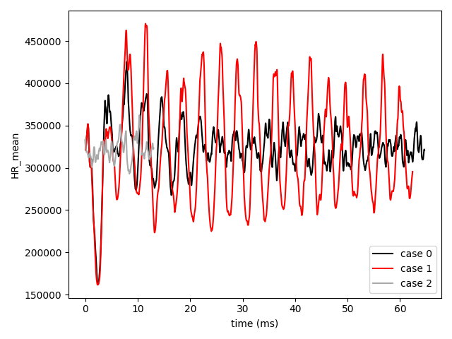
The heat release record of repaired case 2 is short, but still shows amplitudes similar to the reference case 0.
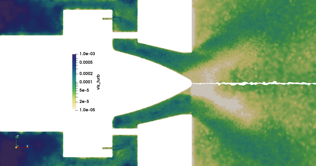
A large eddy simulation rely on the subgrid scale (SGS) model to take into account the turbulence effect at scales smaller than the mesh size. In a Smagorinsky-like model, the SGS expresses as a Turbulent viscosity, controlled both by the flow stress and the mesh size.
In figure 19, the coarsening effect is clearly expressed as an increase of the turbulent viscosity, especially at the injection plane and in the plume of the small fuel injectors before the swirler.
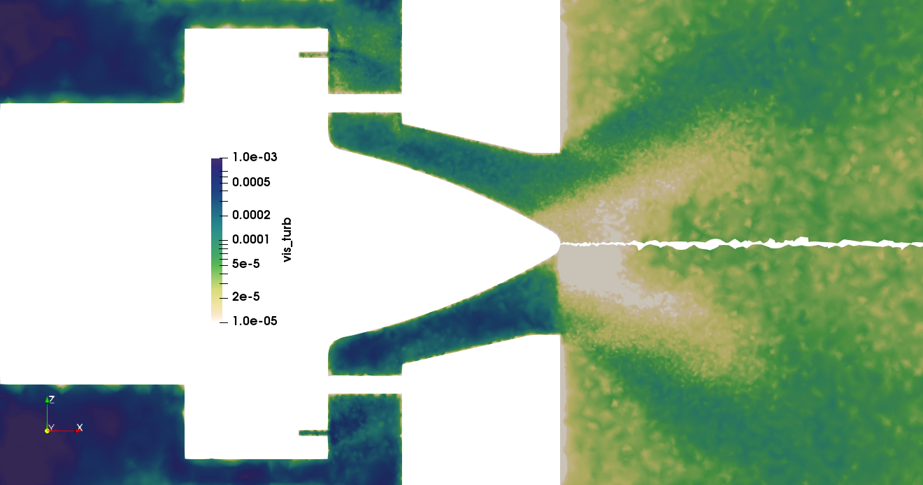
In fig. 20, case 0 and 2 show similar turbulent viscosity fields. The adaptation criteria recovered partly the cell size jump ad the injection level. Case 2 shows also a coarser mesh at the cone tip, because neither LIKE nor Y+ criteria marked this zone for refinement.
The mesh generation workflow converged to a repaired large eddy simulation close to the reference simulation.
Checking the adaptation objectives
It is simple to check a posteriori each constraint. For example, wall modeled turbulence is controlled by the quantity Y+. Fig.21 illustrate how the adaptation adjusted the wall resolution around the required target (Y+= 20).
The mesh generation workflow converged to a wall resolution close to the user-defined target.
Conclusions & perspectives
The present document introduced an automated mesh generation procedure through mesh adaptation.
It demonstrated the capability of this mesh refinement workflow relying on Lemmings and Tekigo within a CFD framework. Apart from the CFD solver, the tools involved are open-source.
The present “aerodynamic” refinement recipe include both a LIKE and y+ criteria. Additional constraints are provided in terms of maximum allowed node number and minimum allowed time step.An important conclusion is that the procedure shows a degree of convergence in the resulting mesh refinements. It could therefore be key in devising a pseudo-meshless strategy for CFD.
This procedure was tested on a mock-up simple geometry for illustration purposes. It can apply several criteria at the same time, and converges to a trade-off between these criteria on a mesh. The final size of the mesh is a user-defined input.
Then the procedure was used on a recent combustion simulation of the PRECCINSTA burner.It converged to a mesh similar to the original one with satisfactory results.
Perspectives
This work will continue in the WP5 of COEC along the following lines.
- The PRECCINSTA simulation on “aerodynamic refined” case 2 will be completed to compare converged statistics on flow fields.
- A similar exercise will be done including a criteria on combustion, with a perturbation/reparation on the flame zone.
- The workflow will test the massively parallel TreeAdapt re-mesher instead of MMG, to create exascale-ready meshes (Over 200 Million cells)
- The pseudo-meshless strategy will also be investigated, focusing on the generation of a primary simple mesh from the CAD.
Disclaimers
The procedure does not include any recommendations on which criteria should be used to create optimal meshes : a large amount of experience and studies is needed to reach a consensus, if any exists.
This procedure is different from a dynamic adaptation technique. Indeed, it targets steady meshes, and thus cannot track flow feature along time, such as shocks, flame fronts or high density gradients. The intermediate meshes and transient computations are considered byproducts of the mesh generation with no CFD meaning, and therefore discarded.
Acknowledgements
The research leading to these results has received funding from the CoEC project under the European Union’s Horizon 2020 research and innovation programme under grant agreement No 952181.
The workflow manager Lemmings has received funding from the Excellerat project under the European Union’s Horizon 2020 research and innovation programme under grant agreement No 823691
Thanks to Gabriel Staffelbach and Jens Mueller for their work on the MMG wrapper in HIP. Thanks also to W. Agostinalli, L. Gicquel and N. Odier for their contributions and comments on the Preccinsta simulations.