![]()
Disclaimer : This post is not finished and has NOT been fully reviewed. Feedback are welcome, but no arguments (yet) please!
Profiling
Most programmers have, at least once, tried to optimise a piece of code, spending hours doing so, only to find in the end that it had virtually no effect on performance, or even that performance had gone down.
To avoid such frustration, and to optimise your time, you need to focus on the parts of the code that really hurt performance. These are called bottlenecks and it is not easy to find them without the right tools. The standard way to do so nowadays is with profiling.
In this blog post we will discuss different tools you can use to profile your python codes.
The basics
The time command
Sometimes you really just need to know if a code is that slow, or how much exactly it is slow. A simple way to figure this out is by using the “time” unix command.
onMacOS$ time python slowHelloWorld.py
Hello World!
python code.py  3,01s user 0,21s system 47% cpu 3,267 total

onUnix$ time python slowHelloWorld.py
Hello World!

real    0m3.014s
user    0m0.211s
sys     0m3.267s
This output can be quite confusing at first. The answer you are probably looking for is the “total” (on macOS) or “real” (on Unix) time. It corresponds to the amount of time your command took from start to completion.
The “user” and “system”/”sys” time are cumulative time the CPU/CPUs spent in user mode or system/kernel mode respectively. These two modes correspond to two levels of privileges. Usually your code runs in user mode, and only asks for kernel mode for specific tasks like file system access.
The total CPU time your code used is the sum of “user” and “sys” time. Note that this time can be less than the “real” time. This happens when your code spent time waiting, for example if it has “sleep” statements, or because the system prioritized an other process over yours. Alternatively, the total CPU time can be larger than the “real” time. This happens when your code runs in parallel since the total CPU time will sum the time of all the cores that worked for you. For parallel codes this can be used to get a rough estimate of efficiency, since in the ideal case the “real” time should be n times smaller than the total CPU time, with n the number of cores you are using.
MacOS users you will also get a fourth value that corresponds to the percentage of CPU used by your code. Note that this is given as a percentage of a single core, for a parallel program this value could be higher than 100%.
The time library
It is essentially an extension of the time command. But instead of timing an entire file, you will be able to get the “real” time for specific blocks of your code.
Its use is extremely simple. Just import the “time” method from the “time” module and use it as a stopwatch. Record the current time before and after the block you want to profile, and take the difference to get its duration in milliseconds.
from time import time

start_time = time()
# block to profile...
stop_time = time()
print("it took", (stop_time-start_time)*1000, "seconds")
Note that it is very handy if you want to profile a very small area of the code, but becomes a mess quickly for big project.
Jupyter notebooks
If you are regularly using jupyter notebooks with an IPython kernel, then you should know about the %time and %%time “built-in magic commands”. These commands give you the CPU “user”, “sys” and “total” time, as well as the “wall” time of the first line of the block, and of the entire block respectively. The “wall” time is the time called “real” or “total” whith the respective Unix and macOS time commands.
In [1]: n = 1000000

In [2]: %time sum_total = sum(range(n))
        sum_even  = sum(_ for _ in range(n) if n%2==0)
        sum_odd   = sum(_ for _ in range(n) if n%2==1)
CPU times: user 20 ms, sys: 928 µs, total: 20.9 ms
Wall time: 20.8 ms

In [3]: %%time
        sum_total = sum(range(n))
        sum_even  = sum(_ for _ in range(n) if n%2==0)
        sum_odd   = sum(_ for _ in range(n) if n%2==1)
CPU times: user 242 ms, sys: 73.1 ms, total: 315 ms
Wall time: 332 ms
Profilers
In this section we will discuss different profilers, how to use them and how to interpret their results.
Most examples will use this file (rec_sum.py) as input code:
from time import sleep

def slow_print(*args, **kwargs):
        sleep(0.001)
        print(*args, **kwargs)

def sum_array(array, acc=0):
        slow_print(len(array))
        if not array:
                return acc
        head, *tail = array
        return sum_array(tail, acc+head)

for i in range(10):
        sleep(0.002)
        sum_array(range(i))
This code recursively computes the sum of the arrays [], [0], [0,1] to [0,1...9] while doing so, it will print 0, then 1,0, then 2,1,0 until 9,8...0.
For some specific explanations we will also use abc.py which is as follows:
from time import sleep

def A():
        B()
        C()
        B()

def B():
        C()

def C():
        sleep(0.01)

A()
This is a very simple program where a function “A” calls “B” 2 times, and “C” 1 times. Internally “B” also calls “C” once. So in the end “C” is called 3 times.
cProfile
cProfile is a built-in library to profile python code. Since it is built-in, you don’t need to install anything. Similarly to many tools, this library can be called in code or in the command line.
Basic usage
You can profile any python code you would launch like this:
python code.py arg1 arg2 arg3
with the following command:
python -m cProfile code.py arg1 arg2 arg3
Please note that this only works with python files, you can’t profile a python CLI by directly calling it:
python -m cProfile my_cli
If you want to profile a CLI, you have to give cProfile the path to the entrypoint. In general, it will be something like this:
python -m cProfile venv/bin/my_cli
Executing this command will output, after the program completion, a table. Each line corresponding to a function called. For example, here is the cProfile of rec_sum.py:
         288 function calls (243 primitive calls) in 0.098 seconds

   Ordered by: standard name

   ncalls  tottime  percall  cumtime  percall filename:lineno(function)
        1    0.000    0.000    0.098    0.098 rec_sum.py:1(<module>)
       55    0.000    0.000    0.074    0.001 rec_sum.py:3(slow_print)
    55/10    0.001    0.000    0.075    0.007 rec_sum.py:7(sum_array)
        1    0.000    0.000    0.098    0.098 {built-in method builtins.exec}
       55    0.000    0.000    0.000    0.000 {built-in method builtins.len}
       55    0.002    0.000    0.002    0.000 {built-in method builtins.print}
       65    0.095    0.001    0.095    0.001 {built-in method time.sleep}
        1    0.000    0.000    0.000    0.000 {method 'disable' of '_lsprof.Profiler' objects}
The first column “ncalls” is the number of times a function was called. Note that there can be two numbers separated by a slash, in this case the second one is the number of “primitive”/”non-recursive” calls, and the first one the total number of calls. Since “sum_array” is a recursive function, we can see that it was called 10 times, but in total, including recursive calls, the code calls this function 55 times. The last column gives the function name as well as its location (filename and line number). Built-in methods are also shown.
Four other columns are present. “tottime” is the cumulated time spent in the function itself, excluding calls to other functions. The column “percall” right next to it is the quotient of “tottime” divided by the total number of calls. “cumtime” is the cumulated time spent in the function, including the calls it did to other functions/subfunctions. The column “percall” right next to it is the quotient of “cumtime” divided by the number of primitive calls.
By default the table is sorted by “standard name”. You can change this with the -s option, giving one of:
calls (call count)
cumulative (cumulative time)
cumtime (cumulative time)
file (file name)
filename (file name)
module (file name)
ncalls (call count)
pcalls (primitive call count)
line (line number)
name (function name)
nfl (name/file/line)
stdname (standard name)
time (internal time)
tottime (internal time)
For example:
python -m cProfile -s time rec_sum.py
gives the table:
         288 function calls (243 primitive calls) in 0.099 seconds

   Ordered by: internal time

   ncalls  tottime  percall  cumtime  percall filename:lineno(function)
       65    0.095    0.001    0.095    0.001 {built-in method time.sleep}
       55    0.002    0.000    0.002    0.000 {built-in method builtins.print}
    55/10    0.001    0.000    0.074    0.007 rec_sum.py:7(sum_array)
       55    0.001    0.000    0.073    0.001 rec_sum.py:3(slow_print)
        1    0.000    0.000    0.099    0.099 rec_sum.py:1(<module>)
       55    0.000    0.000    0.000    0.000 {built-in method builtins.len}
        1    0.000    0.000    0.099    0.099 {built-in method builtins.exec}
        1    0.000    0.000    0.000    0.000 {method 'disable' of '_lsprof.Profiler' objects}
Which clearly points to sleep as the bottleneck of this code… who would have guessed?
Usage in code with pstats
You can get the exact same output as before by importing cProfile and pstats and doing something similar to this:
import cProfile
import pstats

# your code

if __name__ == "__main__":
    with cProfile.Profile() as profiler:
        # call your code
    stats = pstats.Stats(profiler)
    stats.sort_stats(pstats.SortKey.TIME)
    stats.print_stats()
Profile saving
You can save a cProfile profile by using the -o option:
python -m cProfile -o result.prof code.py
This file can be read by other tools.
Snakeviz
As the snakeviz docs says: SnakeViz is a browser based graphical viewer for the output of Python’s cProfile module and an alternative to using the standard library pstats module.
Installation
Snakeviz is a python package you can install as any other package with pip:
pip install snakeviz
Usage
Its usage comes really handy when the table becomes larger and larger. Moreover, it displays additional information about the structure of the code.
First you will have to save a cProfile profile in a file as discussed earlier. Then you can directly call the library with this file:
python -m snakeviz result.prof
This will open a new browser tab with the “call stack” of your code. In this stack, each function is represented by a rectangle which width corresponds to its “cumtime”. The vertical position of the rectangle follows the calls order. Every callee functions sit directly below their caller. As an image is worth a thousand words, here is the snakeviz view of abc.py:
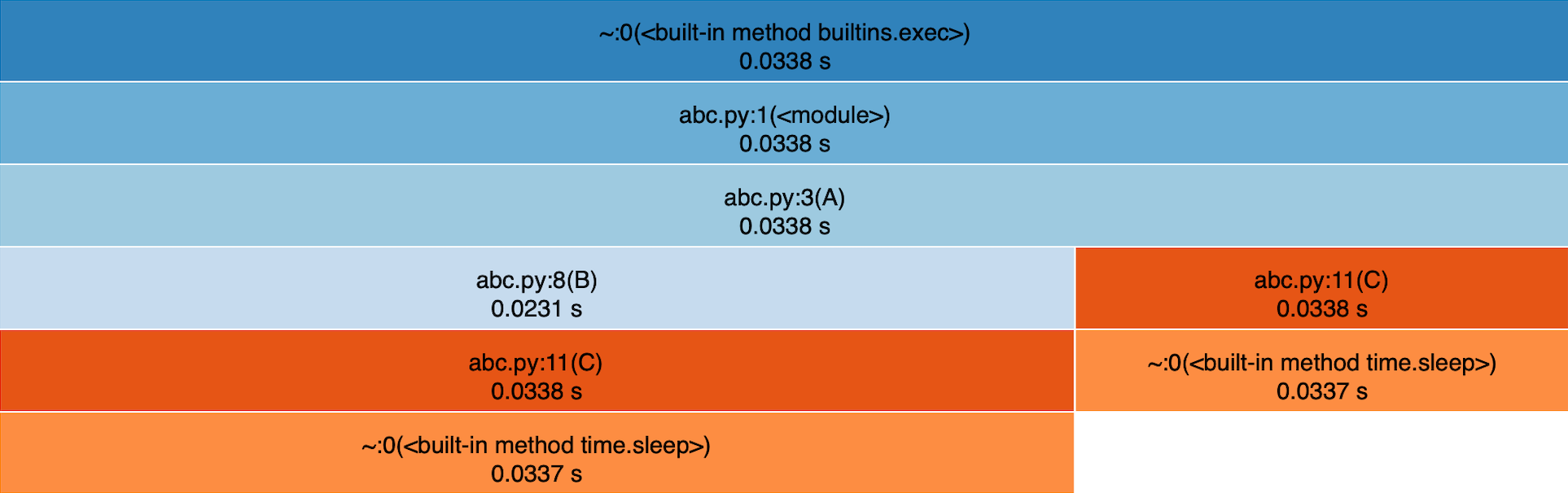
You can clearly see that “A” is at the top, calls “B” and “C”, “B” calls “C”, and “C” calls “sleep”. The thing that can be a bit confusing at first is that snakeviz groups as much as possible the functions. So we lost the fact that “B” was called two times (a single rectangle represents “B”) and the order of calls in “A” (“B”, “C” and “B”).
Here is the rec_sum.py profile and the rest of the interface:
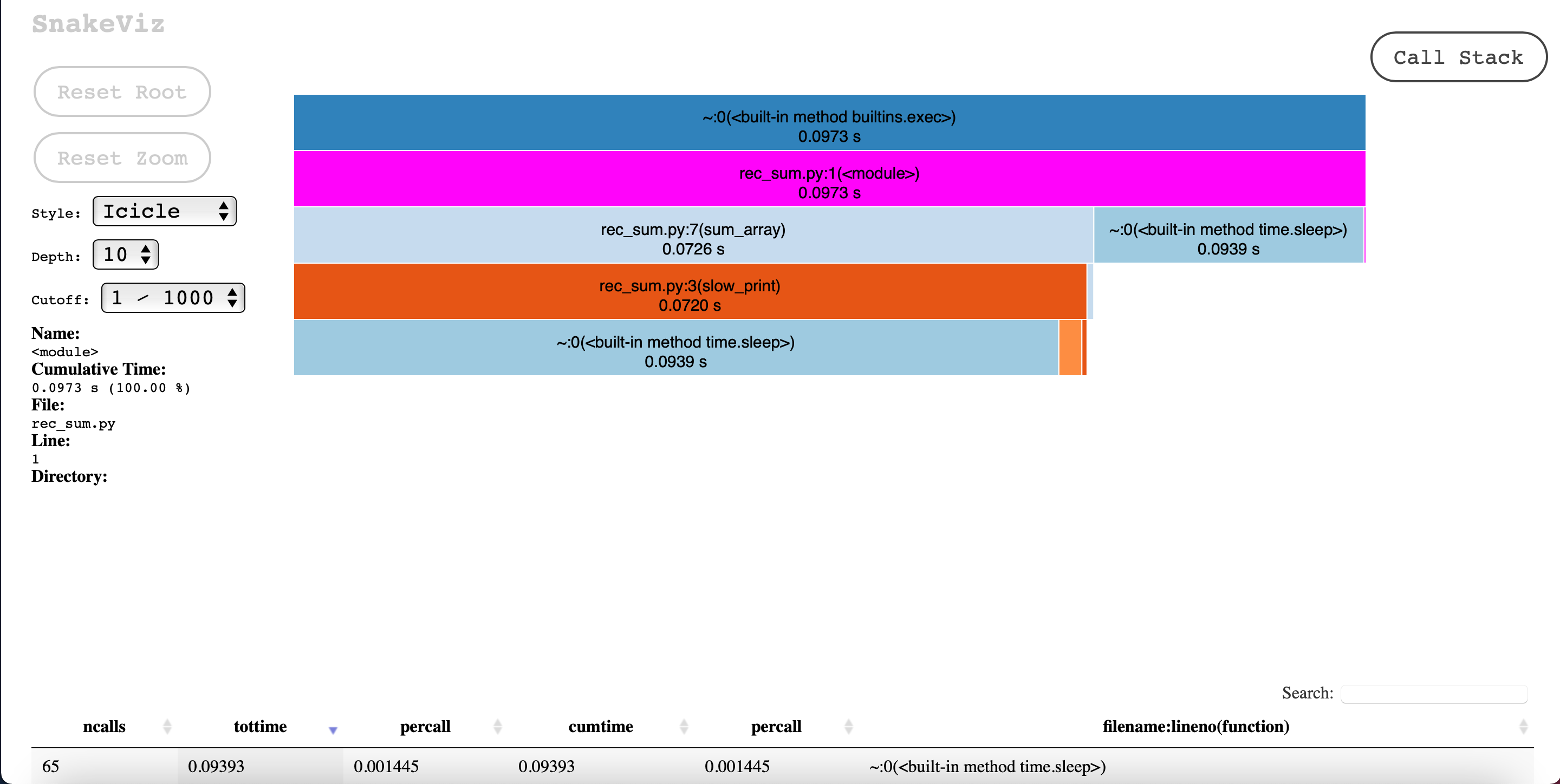
Again, it becomes quite appearant that “sleep” is the bottleneck. It is also very clear that the main source of “sleep” call is “slow_print” in “sum_array”.
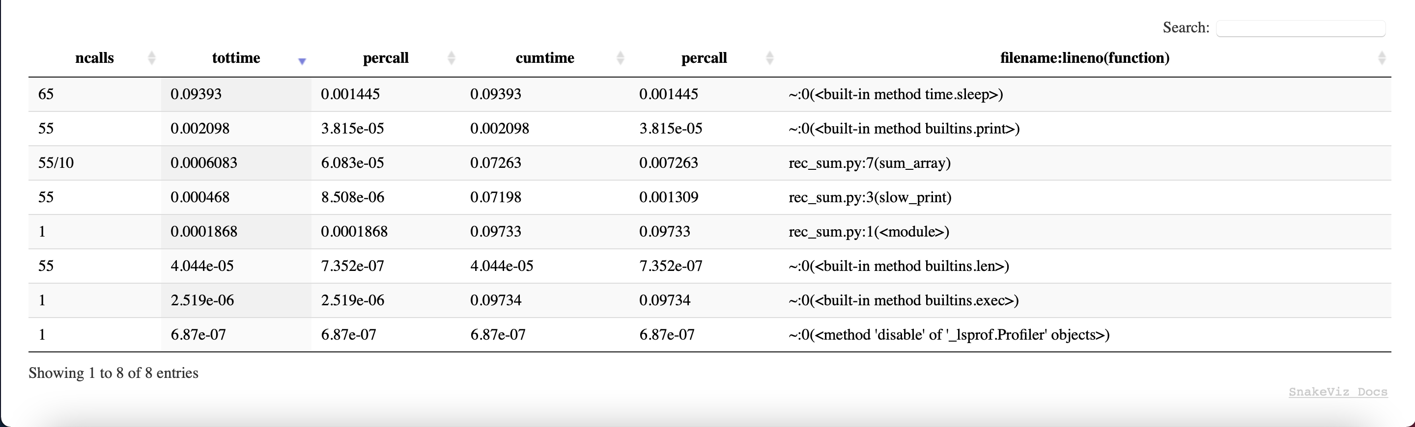
Snakeviz also displays the table we previously discussed. You can order it as you want and even search in it.
Viztracer
Viztracer is also a python package to do profiling. It comes equiped with its own profiler and viewer.
Installation
Viztracer is a python package you can install as any other package with pip:
pip install viztracer
Basic usage
Viztracer comes with a really handy command line interface. You can profile any of your programs by adding “viztracer” at the begining of your command:
viztracer code.py arg1 arg2 arg3
It is worth to mention that viztracer can be used with python CLI without any issues.
The profiling will produce an output file (“result.json” by default). You can change its name by giving a -o option to viztracer:
viztracer -o my_result.json -- code.py arg1 arg2 arg3
The -- is used to delimit viztracer’s arguments and the rest of your command.
Usage in code
Like cProfile, viztracer can be used programmatically. Here is a simple snippet:
from viztracer import VizTracer

# your code

if __name__ == "__main__":
    with VizTracer(output_file="result.json") as tracer:
        # call your code
Vizviewer
Once the json output has been produced you can visualize it with the “vizviewer” command:
vizviewer result.json
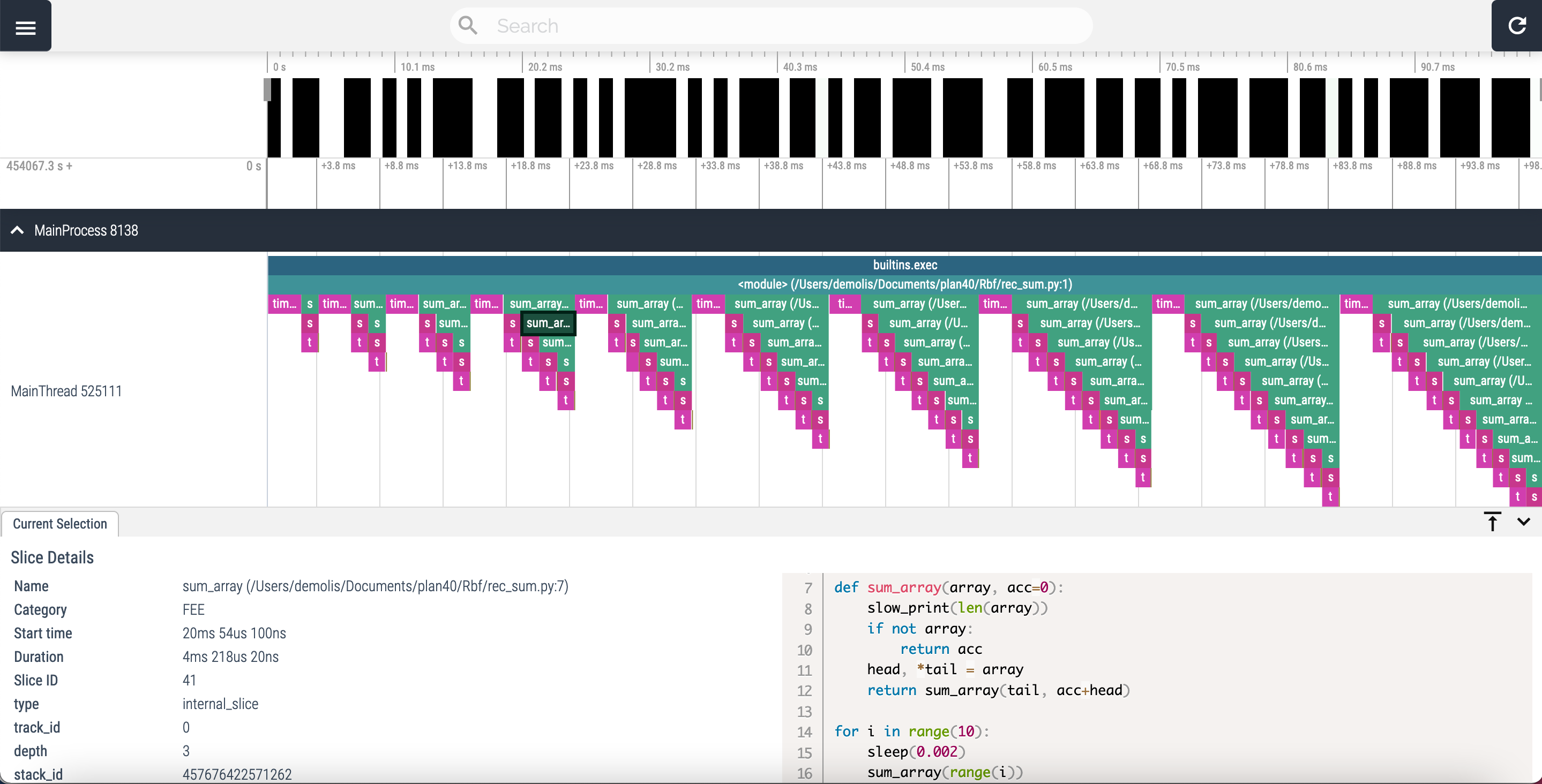
The result will be displayed in a new browser tab:
Please note that you will have to click on “MainProcess” to see anything of interest. Additionally, for large profile, this web interface uses some javascript features that Safari doesn’t support. Chrome and Firefox on the other hand work perfectly well.
Standalone
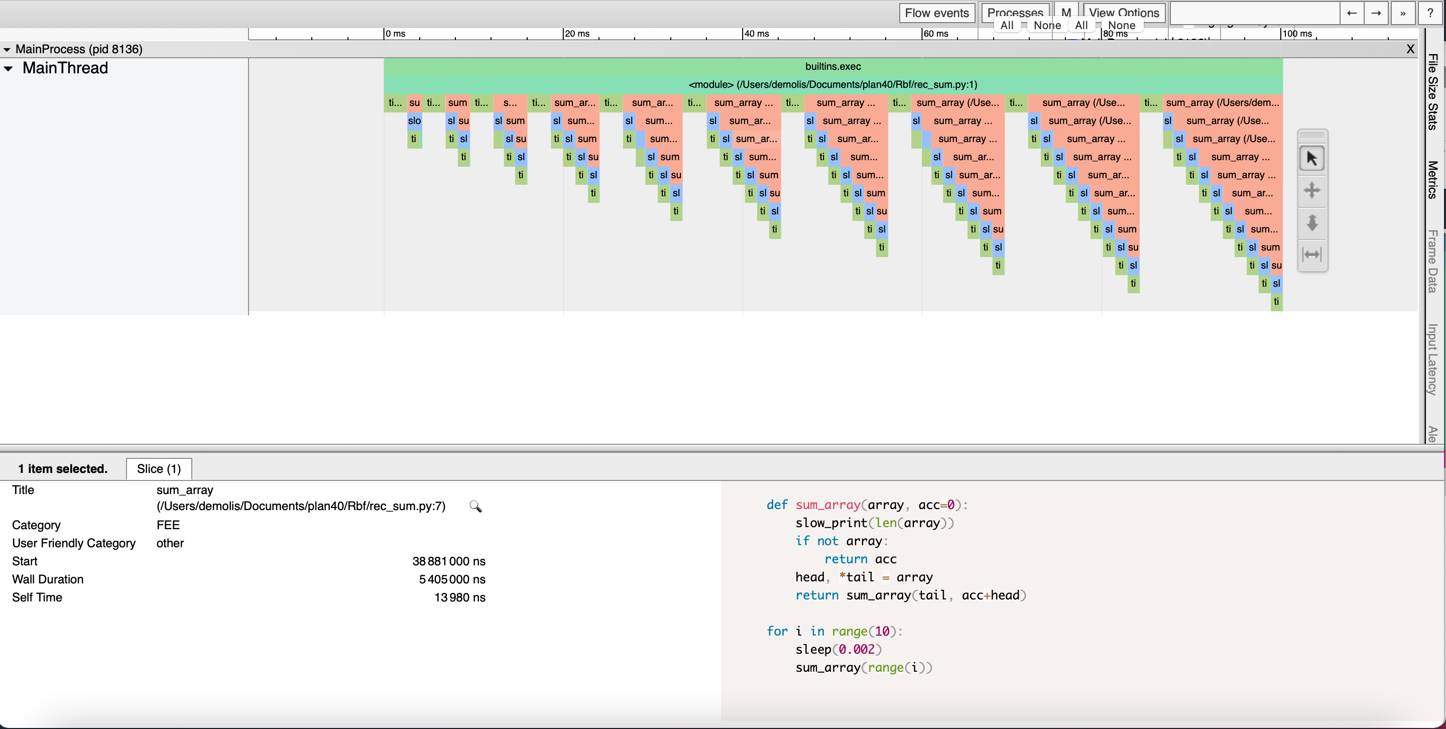
You might want to share your result without having the receiver to install vizviewer, or simply to view the result on Safari or without having to run a web server in the background. You can do so by simply giving an “html” extension to the output file of viztracer:
viztracer -o my_result.html -- code.py arg1 arg2 arg3
The resulting page is mostly similar to the vizviewer version, with roughly the same information but with a less “modern” interface.
Vizviewer interface:
Corresponding standalone:
Understanding the data
Viztracer output can be a little bit overwhelming when lots of data is generated. But the principle is very easy to grasp on little programs.
If you understood how the snakeviz “call stack” works, this should be easy as the principle is quite similar.
Each line on the chart corresponds to a “depth” of execution, and each function is represented by a rectangle placed on the appropriate line which size is defined by its start and stop time. Again, the callee functions are directly below the caller.
Contrary to snakeviz which groups the functions together, each call will be represented separately in viztracer. Here is the abc.py profile:
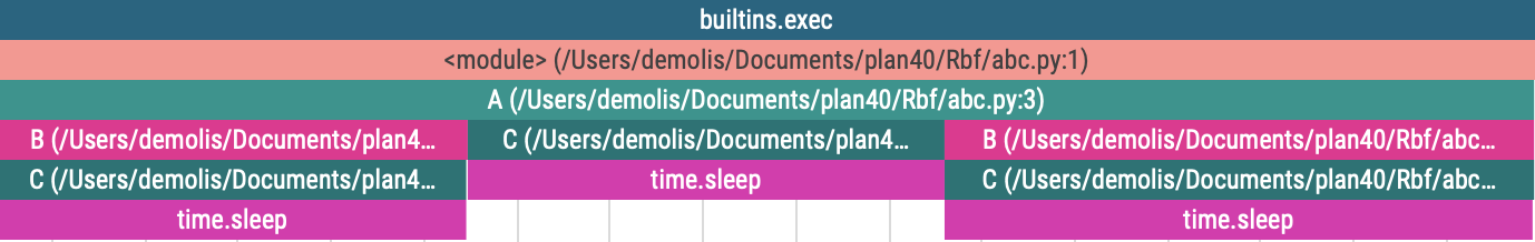
Here we can clearly see that “A” calls “B”, then “C” and “B” again.
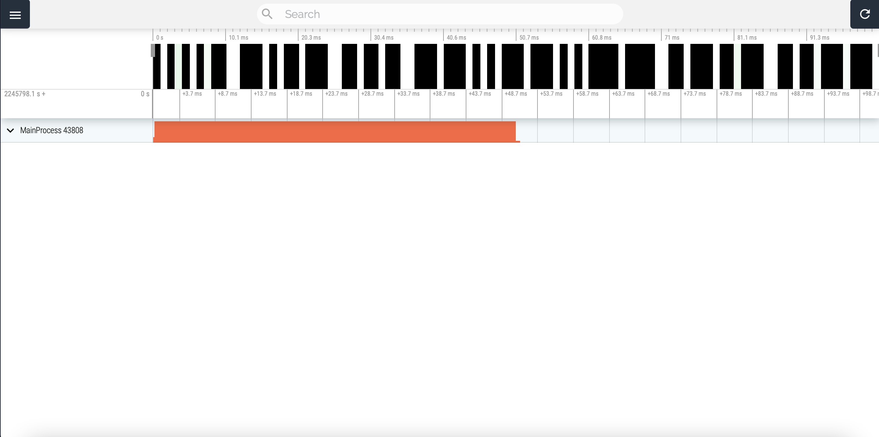
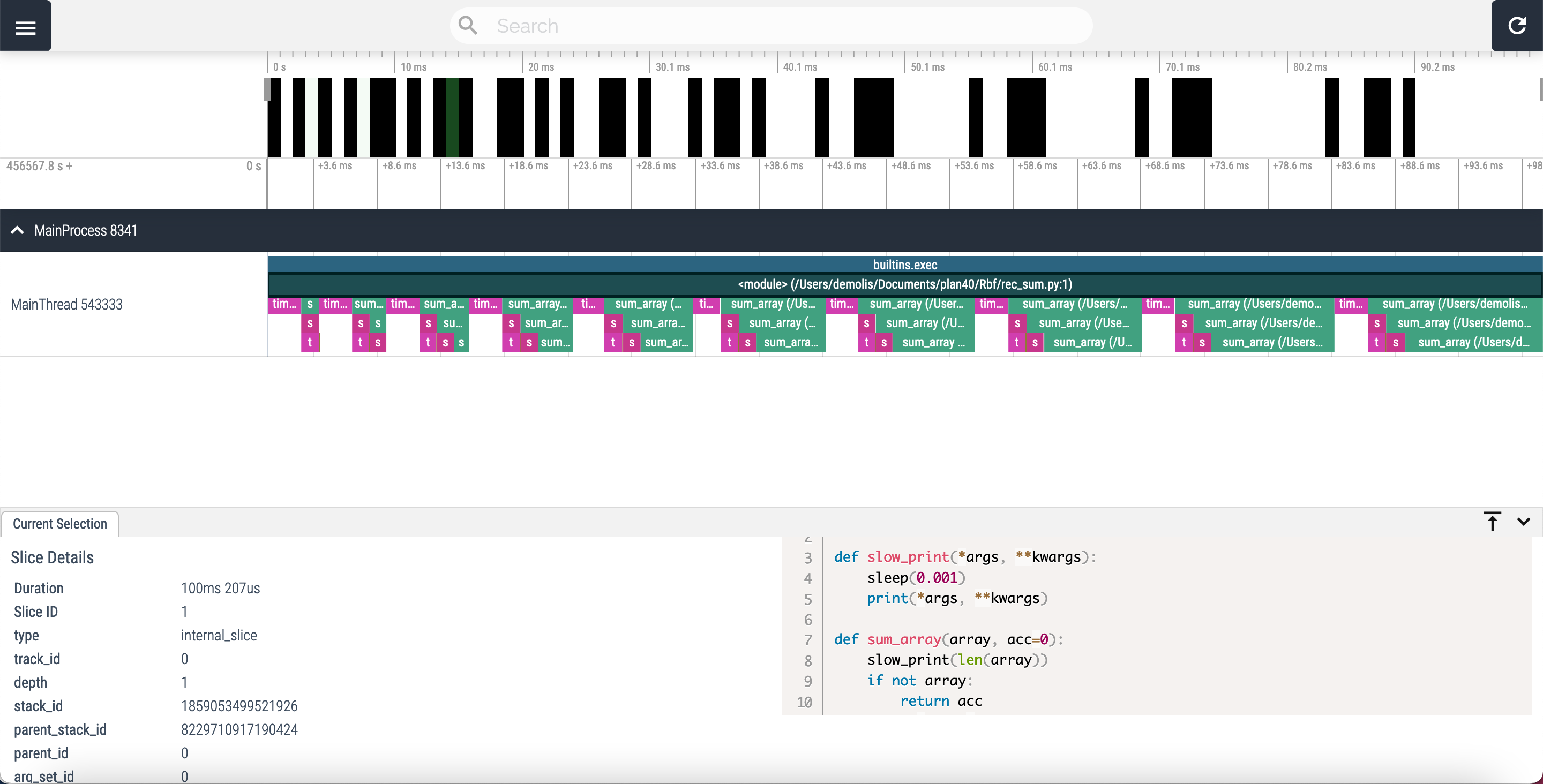
The same goes for rec_sum.py profile:
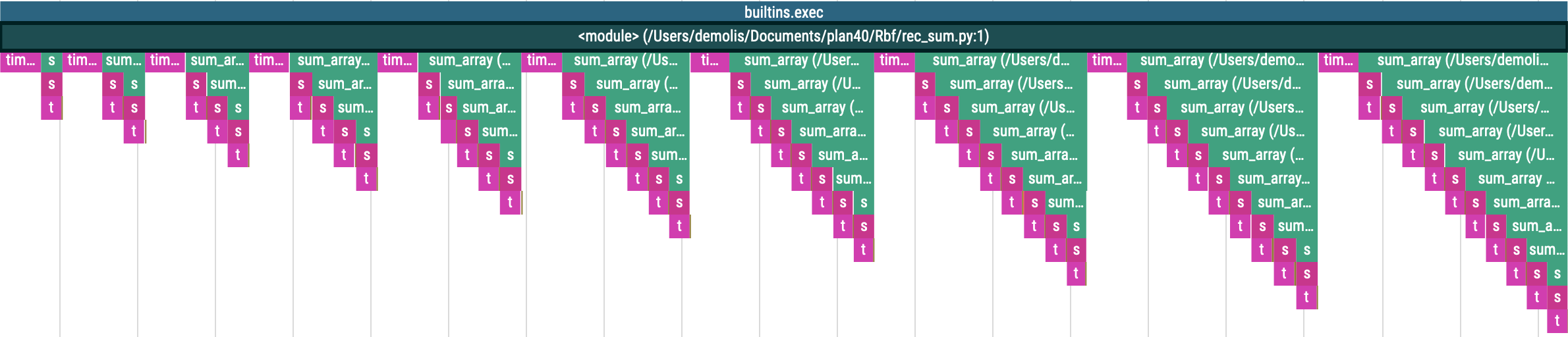
Each iteration of the main for loop produces a “triangle” on the chart. Each triangle representing the recursive nature of the “rec_sum” function.
Line by line using line_profiler
Sometimes you need a sharper picture. line_profiler allows this, with the great advantage of profiling only the part you need.
To profile a python script:
Install line_profiler: pip install line_profiler.
In the relevant file(s), import line profiler and decorate function(s) you want to profile with @line_profiler.profile.
Set the environment variable LINE_PROFILE=1 and run your script as normal. When the script ends a summary of profile results, files written to disk, and instructions for inspecting details will be written to stdout.
The results looks like:
Timer unit: 1e-06 s

Total time: 0.731624 s
File: ./demo_primes.py
Function: is_prime at line 4

Line #      Hits         Time  Per Hit   % Time  Line Contents
==============================================================
     4                                           @profile
     5                                           def is_prime(n):
     6                                               '''
     7                                               Check if the number "n" is prime, with n > 1.
     8
     9                                               Returns a boolean, True if n is prime.
    10                                               '''
    11    100000      14178.0      0.1      1.9      max_val = n ** 0.5
    12    100000      22830.7      0.2      3.1      stop = int(max_val + 1)
    13   2755287     313514.1      0.1     42.9      for i in range(2, stop):
    14   2745693     368716.6      0.1     50.4          if n % i == 0:
    15     90406      11462.9      0.1      1.6              return False
    16      9594        922.0      0.1      0.1      return True
Remarks
Vizviewer can’t handle too much data. So for huge project or higly repeating/recursive programs, the amount of data generated can crash the visual tool. A drastic way to reduce the data to display and to analyse is to limit the stack depth:
viztracer --max_stack_depth arg -- code.py arg1 arg2 arg3
This direclty cuts down the number of lines on the chart.
The profile of rec_sum.py with a max_stack_depth set to 5, looks like this:
Viztracer offers tons of options, a lot can be used to include/exclude function calls on the chart. For more information please check the package doc here.
Conclusion
Python offers a multitude of tools for profiling your code, many more than I have discussed in this post. Some are native, others need to be installed. All have advantages and disadvantages. Many programmers are still stuck with the first methods described (time library in particular), but as said earlier, these methods don’t scale well at all. Even if the graphs and tables produced by profilers can seem intimidating, I encourage you to try one now. Once you are familiar with their format, the insights you will be able to get from them are invaluable.