Calculate profiles on AVBP cuts with PyAVBP

Introduction

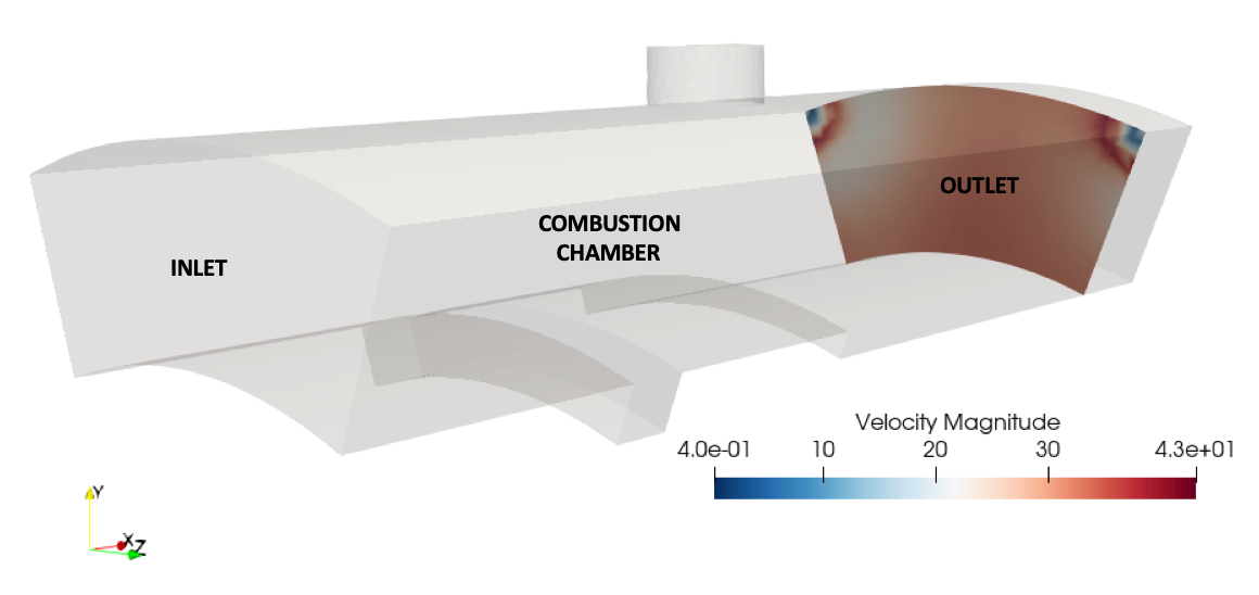
PyAVBP is an API for CERFACS’s AVBP software. AVBP has many features to simulate the behaviour of an engine’s combustion chamber. In a gas turbine, the combustion chamber is upwind the turbine. The turbine is a high speed rotating part submitted to high temperature air flux. Such level ot thermo-mechanical constraints supposes a complex design in order to achieve its purpose of recovering mechanical energy. A good description of the airflow at the outlet of the combustion chamber is extremely important. That is why PyAVBP proposes the module shell_average_profiles.

shell_average_profile module

This module aims at analyzing a bunch of cuts at the outlet of the combustion chamber. It gets the fields of temperature, density, velocity, etc., and makes an integration across different dimensions.

The field can be integrated:

• over time to get a temporal average map:

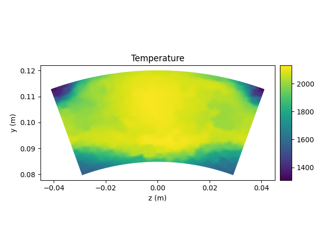
• over time and azimuthally to get the temperature profile in the height of the cut:

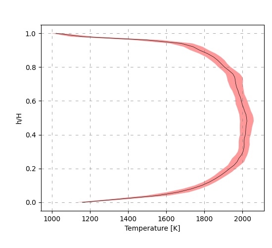
• over the two spatial directions of the cut to get the temporal evolution of the spatial mean:

• over time and space to get a mean value.

Usecase

Imagine we have the results of a CFD simulation. We have the cuts of the outlet of the combustion chamber in a folder POSTPROC. First we import everything we need:

from pyavbp.tools import shell_average_profiles as sap
from pyavbp.tools.cut_utils import ShellParams
from pyavbp.tools.cut_utils import infer_shell_from_cuts

The module shell_average_profiles contains the main functions to calculate several fields. The class ShellParams is a necessary object to create the shell on which we will interpolate our solutions while infer_shell_from_cuts is the function that will create the shell.

Define the location of your cut files:

solution_paths = 'POSTPROC/'
solution_prefix = 'outlet_vortex_cut_cut'

Now you need to create the shell. In fact, calculate_profiles_on_shell is based on an adapted version of the mesh called a shell, that is to say a structured mesh.

shell = infer_shell_from_cuts(
        solution_paths,
        solution_prefix,
        ShellParams("axicyl", 41, 41))

infer_shell_from_cuts takes three arguments. The two first arguments are related to the location of the solutions. The third one is a ShellParams object. At instanciation, a ShellParams takes the type of shell (either “axicyl” or “cart”), n_u and n_v (number of discretization points in each direction r and θ). Now that you have your shell -or structured mesh-, you can call the function that will calculate all the interpolated profiles and pack them into a dict:

profiles = sap.calculate_profiles_on_shell(solution_paths,
                                     solution_prefix,
                                     shell_params)

Now you can either use the results to:

• make treatments on them:

print(profiles.keys())
>dict_keys(['2D', '1D', '1D_temporal', '0D'])
print(profiles['1D_temporal'].keys())
>dict_keys(['T_avg', 'T_avg_max', 'idx_T_avg_max', 'T_max', 'idx_T_max', 'FAR', 'MassFlow', 'Time'])
profiles['1D_temporal']['T_avg_max']
...

• dump them in a directory:

sap.dump_profiles(shell, profiles, 'png', 'csv')

Like this post? Share on: Twitter ❄ Facebook ❄ Email