
Plane Shear Layer Initialization
The following treatment creates the mesh and the initial condition for a plane shear layer.
Parameters
- domain_size: list(float)
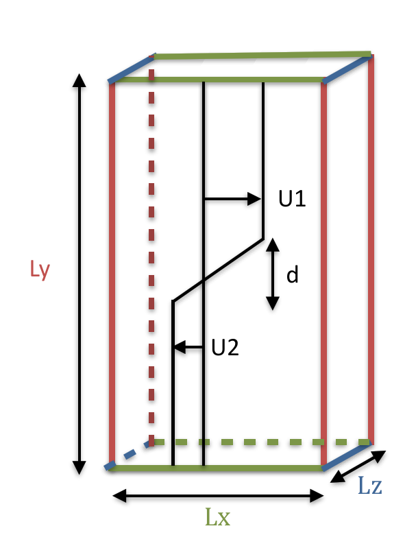
Size of the box in longitudinal (Lx), normal (Ly), and transverse (Lz) directions.
- mesh_node_nb: list(int)
Number of nodes used to create the mesh in the longitudinal (Nx), normal (Ny), and transverse (Nz) directions.
- base_flow_velocities: list(float)
Base-flow velocities up and down the shear-layer.
- shear_layer_thickness: float
Thickness of the shear layer to meet top to down base-flow velocities.
- perturbation_amplitude: float
Amplitude of the perturbation related to the exponential term.
- inf_state_ref: list(float)
Conservative variables at infinity.
Preconditions
Perfect Gas Assumption: \(\gamma=1.4\).
Main functions
- class antares.treatment.init.TreatmentInitShearLayer.TreatmentInitShearLayer
- execute()
Compute an initial field with a shear.
The returned base contains one structured zone with one instant with default names. It contains a structured mesh and conservative variables (ro, rou, rov, row, roE) at nodes.
The flow field is composed of a base flow based on a uniform velocity \(U_1\) for \(y > \frac{d}{2}\) and \(U_2\) for \(y< -\frac{d}{2}\).
In the shear layer domain (\(-\frac{d}{2} < y < \frac{d}{2}\)), the base flow profile is a linear profile that ensures velocity continuity between the two uniform domains.
\(U(y) = U_1\) for \(y \geq \frac{d}{2}\)
\(U(y) = \frac{U_1-U_2}{d} y + \frac{U_1-U_2}{2} y\) for \(-\frac{d}{2} < y < \frac{d}{2}\)
\(U(y) = U_2\) for \(y \leq \frac{d}{2}\)
A perturbation is added to the base flow:
\(u_1 = \alpha B \exp(-\alpha y) \sin(\alpha x), v_1 = \alpha B \exp(-\alpha y) \cos(\alpha x)\) if \(y \geq 0\)
\(u_2 = \alpha B \exp(-\alpha y) \cos(\alpha x), v_2 = \alpha B \exp(-\alpha y) \sin(\alpha x)\) if \(y < 0\)
with \(\alpha = \frac{2 \pi}{\lambda}\), \(\lambda\) being the perturbation wavelength.
Example
import os
if not os.path.isdir('OUTPUT'):
    os.makedirs('OUTPUT')

import antares

t = antares.Treatment('InitShearLayer')
t['domain_size'] = [1.0, 1.0, 1.0]       # [Lx,Ly,Lz]
t['mesh_node_nb'] = [20, 20, 20]         # [Nx,Ny,Nz]
t['base_flow_velocities'] = [10.0, 6.0]  # U1 et U2 velocities
t['shear_layer_thickness'] = 0.1         # shear layer thickness (d)
t['perturbation_amplitude'] = 0.0005     # Coefficient B
t['inf_state_ref'] = [1.16, 0.0, 0.0, 0.0, 249864.58]
b = t.execute()

print(b[0][0])
w = antares.Writer('hdf_antares')
w['base'] = b
w['filename'] = os.path.join('OUTPUT', 'ex_test')
w.dump()