Plot bases ¶

Description ¶

This treatment provides a flexible way to render bases using the VTK library. Each base can be visualized either by coloring its geometric zones or by mapping one of its scalar variables to a color scale. Multiple bases can be rendered simultaneously, each using a different variable for coloring. Additionally, a list of 3D points can be displayed as spheres .

The treatment supports both interactive visualization and off-screen rendering, making it suitable for both exploratory analysis and automated batch processing.

The scenes are fully customizable, with support for adjusting colorbars and visual aesthetics, adding text or image annotations, and setting precise camera positions to control the viewpoint.

New in version 2.5.0.

Parameters ¶

bases: Base or list(Base)
The input base or bases to be shown
zones: list(str) or list(int), default= None
The name or indexes of zones to plot. It is assumed all bases have all zones. If None, plot all zones.
instants: list(str) or list(int)
The name or indexes of instants to plot. It is assumed all bases have all instants. If None, plot all instants.
time_start: float, default: 0.0
The physical time of the first instant
time_step: float, default: 1.0
The timestep between two instants.
figindex_start int, default: 0
The starting index of the figures to be saved
show_mesh bool, default: False
Whether to show the base mesh or not
mesh_color str, default: 'black'
The color of the mesh lines (see Colors for more details).
mesh_linewidth float, default: 3.0
The with of the mesh lines
color_by: str, default: 'zones'
The variable to be plotted. If color_by = 'zones', show the base’s zones. If color_by = 'in_attr', use the base attributes to extract the treatment’s arguments. See XXX
zone_colors: str or dict, default: 'cycle'.
If color_by == 'zones', then this arguments specifies how the zones are colored. It can be a string with the color name, in which case all zones are colored with the same color. It can be a dictionary whose keys are the zones names and the values are the colors. Or it can be 'cycle', in which case the zones colors will cycle through the list ['blue', 'orange', 'green', 'red', 'purple', 'pink', 'cyan']
transparency: float, default: 0.0
A value between 0 and 1 specifying the base’s transparency.
- 0 = no transparency
- 1 = full transparency (base will not be visible)
colorbar: bool, default: True
Whether to show the colorbar or not.
colorbar_range str or list, default: 'auto'
The min-max values of the color bar, in the form of [min, max]. If 'auto', the treatment will compute the min and max values by checking every zone and instant of each base to be plotted with such variable.
colorbar_nb_labels int, default: 6
The number of labels in the color bar.
colorbar_height int or str, default: 'auto'
The height of the color bar in relative units to the figure size. colorbar_height = 1 means the bar height is equal to the figure height. If 'auto', the height will be set to 0.6 for vertical bars, and to 0.1 for horizontal bars.
colorbar_width int or str, default: 'auto'
The width of the color bar in relative units to the figure size. colorbar_width = 1 means the bar width is equal to the figure width. If 'auto', the width will be set to 0.1 for vertical bars, and to 0.6 for horizontal bars.
colorbar_position list(float) or str, default: 'auto'
The position of the colorbar in relative units (see Relative coordinates). If 'auto', the position will be (0.2, 0.1) for horizontal bars, and (0.8, 0.2) for vertical bars.
colorbar_horizontal bool, default: False
If True sets the colorbar orientation to horizontal
colorbar_boldfont bool, default: False
If True sets the colorbar font to bold.
colorbar_labelformat str, default: '%g'
Sets the numeric format for the colorbar labels. The format must be specified in C-style format strings. Here are a few examples:
- '%.2f': Float numbers with 2 decimal values (323.23)
- '%.3e': Scientific notation with 3 decimal values (3.232e+02)
- '%d': Integer value (323)
- '%g': It chooses between '%f' and '%e' automatically depending on the values.
colorbar_title str, default: '{var}'
Set’s the title of the colorbar. A placeholder '{var}' can be used to set the title equals to the name of the variable plotted.
colorbar_title_fontsize float, default: 36.0
The colorbar’s title fontsize.
colorbar_title_fontcolor str, default: 'color'
The colorbar’s title font color (see Colors for more details).
colorbar_title_boldfont bool, default: False
If True sets the colorbar’s title font to bold.
colorbar_title_fontfamily str, default: 'times'
Sets the colorbar title font family (see Font families).
colorbar_title_fontname str, default: None
Sets a custom font for the colorbar’s title from the installed fonts in your system (see Font families).
colorbar_ticks_fontsize float, default: 36.0
The colorbar’s ticks fontsize.
colorbar_labels list(float) or list(tuple(str, str)), default: None
The labels to be shown in the colorbar (see Colorbar labels).
colorbar_ticks_fontcolor str, default: 'color'
The colorbar’s ticks font color (see Colors for more details).
colorbar_ticks_boldfont bool, default: False
If True sets the colorbar’s ticks font to bold.
colorbar_ticks_fontfamily str, default: 'times'
Sets the colorbar tick font family (see Font families).
colorbar_ticks_fontname str, default: None
Sets a custom font for the colorbar’s ticks from the installed fonts in your system (see Font families).
colorbar_discrete bool, default: False
Use a discrete colorbar instead of a continuous one
colorbar_discrete_nb_values int, default: 8
Number of discrete values in a discrete colorbar
colormap str, default: 'rainbow_uniform'
The colormap use to plot the variable (See Colormaps for more details).
colormap_invert bool, default: False
Whether to invert the chosen colormap or not.
nan_color str, default: 'magenta'
Color use to render NaN values.
point_show_labels bool, default: False
If True, show a text label next to each point.
point_labels str or dict, default: 'global'
Set’s the labels displayed. If 'global', points are numbered globally and their index is displayed as the label. If 'base' each point within a base is numbered and their index is displayed as the label. If 'zone', each point within base[zone] is numbered and their index is displayed as the label. Custom labels can also by specified using a dictionary. The key of the dictionary must be the zone names in the base and the value is a list of strings with the label assigned to each point in the zone.
point_label_offset float or list(float), default: 0.05
The label of each point is displayed at the position of the point plus an offset. If point_label_offset is a single float, the offset is applied equally in all directions. Otherwise, the user can specify the offset in the three directions [offset_x, offset_y, offset_z].
point_label_fontsize float, default: 36
The font size of the point labels
point_label_color str, default: 'black'
The font color of the point labels (see Colors)
point_fontfamily str, default: 'times'
The font family for the point labels.
point_fontname str, default: Name
Sets a custom font for the point labels from the installed fonts in your system (see Font families).
axes bool, default: True
Whether to show the coordinate axes or not.
axes_labels list(str), default: ['X', 'Y', 'Z']
A list of strings with the axes labels.
axes_colors list(str), default: ['red', 'green', 'blue']
A list of strings with the axes colors
axes_position list(float), default: [0.1, 0.1]
The axes position in relative coordinates (see relative coordinates)
axes_size float, default: 0.2
The axes size.
axes_linewidth float, default: 1
The axes line width.
axes_fontsize float, default: 24
The axes font size.
axes_fontcolor str, default: 'black'
The axes font color (see Colors).
axes_fontfamiles str, default: 'times'
The axes font family (see Font families).
axes_fontname str, default: None
Sets a custom font for the axes from the installed fonts in your system (see Font families).
texts dict, default: {}
Texts to be inserted in the figure (see Inserting text).
images dict, default: {}
Images to be inserted in the figure (see Inserting images).
figsize list(int) or str, default: [1280, 720]
Either a list of two values representing [width, heigh] of the figure. Or a string to the path of the camera settings.
background_color str, default: 'white'
The image background color (see Colors for more details). It can also accept as value: “transparent”, for transparent backgrounds.

Warning

Only PNG images handle transparent backgrounds
camera_position list(float), default: None
The position of the camera. If None, use VTK default.
camera_focal_point list(float), default: None
The point the camera is looking at. If None, use VTK default.
camera_view_up list(float), default: None
The “up” direction of the camera view. Must not be parallel to the view direction. If None, use VTK default.
camera_zoom float, default: None
Zoom factor. A value >1 zooms in, <1 zooms out. Works in both perspective and parallel modes.
camera_angle float, default: None
Vertical field of view in degrees. Used only in perspective projection.
camera_parallel_projection bool, default: False
Whether to use parallel (orthographic) projection instead of perspective.
camera_direction: str or list(float), default: 'iso'
A string or list that sets the predefined view direction of the camera. If it’s a string it must be one of the followings:
- ‘X+’: camera looks in the X+ direction
- ‘X-’: camera looks in the X- direction
- ‘Y+’: camera looks in the Y+ direction
- ‘Y-’: camera looks in the Y- direction
- ‘Z+’: camera looks in the Z+ direction
- ‘Z-’: camera looks in the Z- direction
- ‘iso’: Isometric 3D view, where camera is positioned in [1, 1, 1] looking towards the origin
If it is a list, it must be a list of 3 floats with the position of the camera. The camera will look from that points towards the origin and an automatic camera reset will be enforced to ensure all bases are visible.
camera_force_reset bool, default: False
Whether to force the a full camera reset after setting the camera’s properties. A camera reset ensures that all objects will be visible.
camera_save_settings str, default: None
Filename to save the camera properties and window’s size each time the user interacts with the window.
camera_load_settings str, default: None
Filename to read the camera properties (It does not read the figure size, use figsize for that).
show: bool, default: false
if true, opens an interactive window with the rendering.
output_file: str, default: None
The filename to save the image. It must ends in either “.png”, “.jpeg” or “.jpg”. If show == True, then the image saved is the last imaged shown in the window. The strings accepts the following placeholders:
- {instant}: The current instant name
- {figindex}: The current fig index
- {var}: The variable being plotted.
memory_mode bool, default: False
If True, delete each instant from memory after the plot is done.
progress_bar bool, default: False
If True, shows a progress bar.
progress_bar_label str, default: 'Plotting bases'
The label of the progress bar.
jupyter bool, default: False
If you are in a jupyter session, set this to True to show the image in the notebook.

Preconditions ¶

The treatment assumes the following

All bases to be plotted must be unstructured bases.
All bases to be plotted have the same instants (but they don’t need to have the same zones)
Variables to be plotted are on nodes

Postconditions ¶

If 'memory_mode' = True, the plotted instants will be removed from the bases.

Plot variables ¶

Single base plotting ¶

If only a single base is to be plotted, you can use the bases and color_by keywords to specify which base and which variable to visualize. Visual properties such as show_mesh, mesh_color, mesh_linewidth, and transparency should be defined using the treatment’s keywords. Colorbar customization is handled using the colorbar_* keywords,

treatment['bases'] = base
treatment['color_by'] = 'rho'
treatment['colorbar'] = True
treatment['colorbar_title'] = r'$\rho$'
# ...
treatment.execute()

Multiple bases with the same variable ¶

If multiple bases are to be plotted using the same variable, you must provide the list of bases using the bases keyword. The color_by keyword specifies which variable is plotted across all selected bases.

Visual customization options such as show_mesh, mesh_color, mesh_linewidth, and transparency must be defined in each base’s attributes. This is done by adding a base attribute named plotbases, which is a dictionary mapping treatment-level keywords to their corresponding values.

In this setup, colorbar properties can also be specified using any of the colorbar_* keywords within the plotbases dictionary to control the colorbar appearance.

# For the first base we show the mesh in red as well
base1.attrs['plotbases'] = {
 'show_mesh': True,
 'mesh_color': 'red',
 'mesh_linewidth': 1,
}

treatment['bases'] = [base1, base2]
treatment['color_by'] = 'rho'
treatment['colorbar'] = True
treatment['colorbar_title'] = r'$\rho$'
# ...
treatment.execute()

Multiple bases with different variables ¶

If you need to plot multiple bases, and each base should display a different variable, you must set color_by to 'in_attr'. In this mode, each base’s attributes determine which variable is plotted.

As in the example above, visual properties like show_mesh, mesh_color, mesh_linewidth, and transparency can be specified within each base’s attributes.

Colorbar customization is handled similarly. The colorbar_* keywords should be included in each base’s attributes to control the colorbar for that specific base. You can also use the treatment-level colorbar_* keywords to set default colorbar settings that apply to all variables.

When two or more bases plot the same variable, only one colorbar is displayed for that variable. The properties of that colorbar are determined by merging the colorbar_* settings from all relevant bases. If multiple bases define the same colorbar property, the value from the last base in the list takes precedence.

base1.attrs['plotbases'] = {
  'transparency': 0.5,
  'color_by': 'rho',
  'colorbar': True,
  'colorbar_title': r"$\rho$",
  'colorbar_horizontal': True,
  'colorbar_labelformat': '%.2f' # Custom label for density colorbar
}

base2.attrs['plotbases'] = {
  'show_mesh': True,
  'color_by': 'pressure',
  'colorbar': True,
  'colorbar_title': r"$P$",
  'colorbar_horizontal': False,
}

treatment['bases'] = [base1, base2]
treatment['color_by'] = 'in_attr'
treatment['colorbar'] = True
treatment['colorbar_title'] = r'$\rho$'
treatment['colorbar_nb_labels'] = 2 # Both colorbars will have only 2 labels
treatment['colorbar_labelformat'] = '%.2e' # Scientific notation with 2 decimals
# ...
treatment.execute()

Showing list of points ¶

If the base has no connectivity, it will be rendered as a collection of individual spheres. Each point can be colored either by any variable available in the base or by its corresponding zone. The size of the points is controlled by the point_radius parameter.

Labels can be displayed next to each point if point_show_labels is set to True. The content of these labels is defined by the point_labels option, which supports the following modes:

global: Each point is assigned a unique number across the entire dataset.
base: Each point is assigned a unique number within its base.
zone: Each point is assigned a unique number within its base and zone.

Labels are positioned at the point’s location, with an optional offset specified by point_label_offset. Additional styling options for the labels—such as font size, font family, and color—can also be customized.

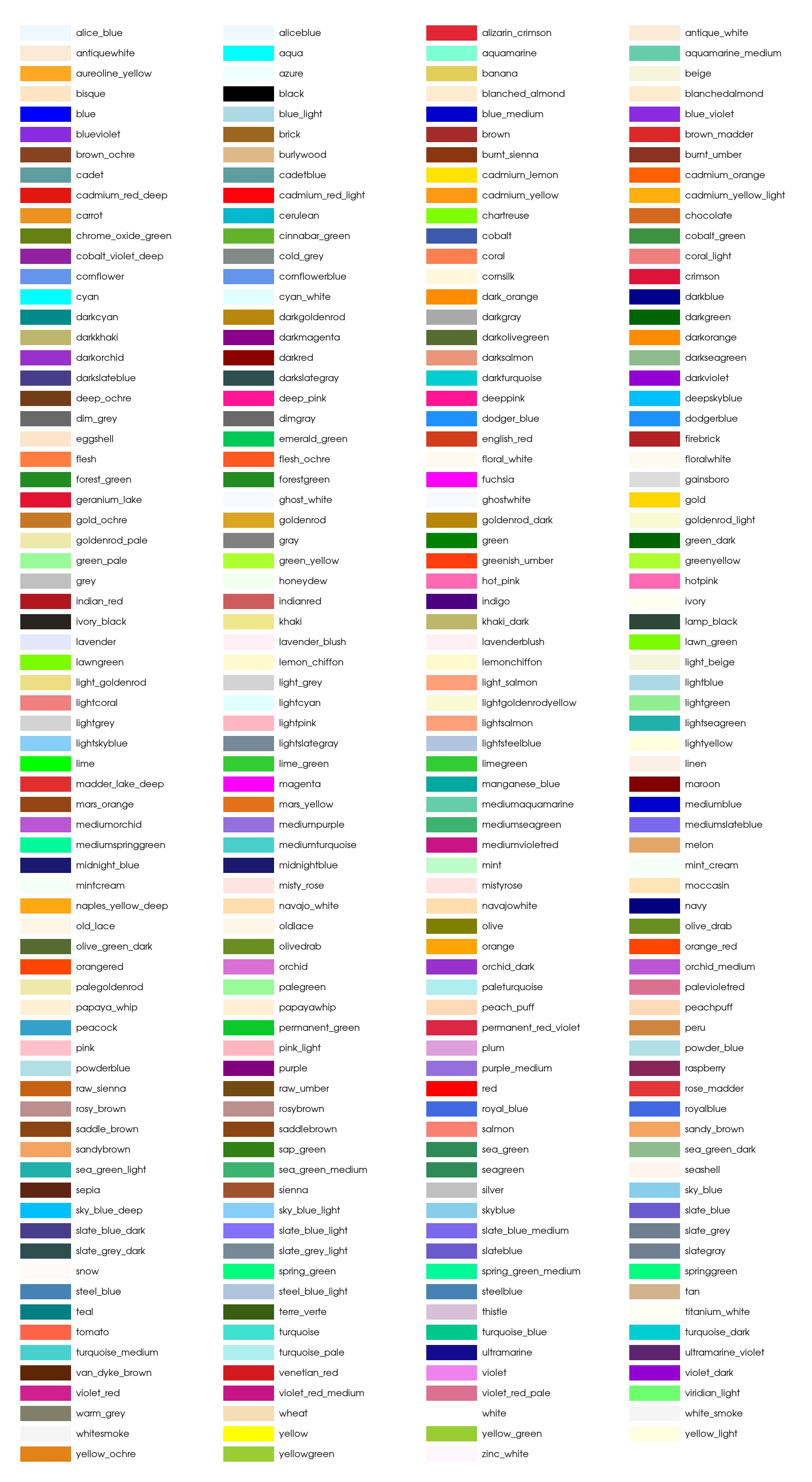
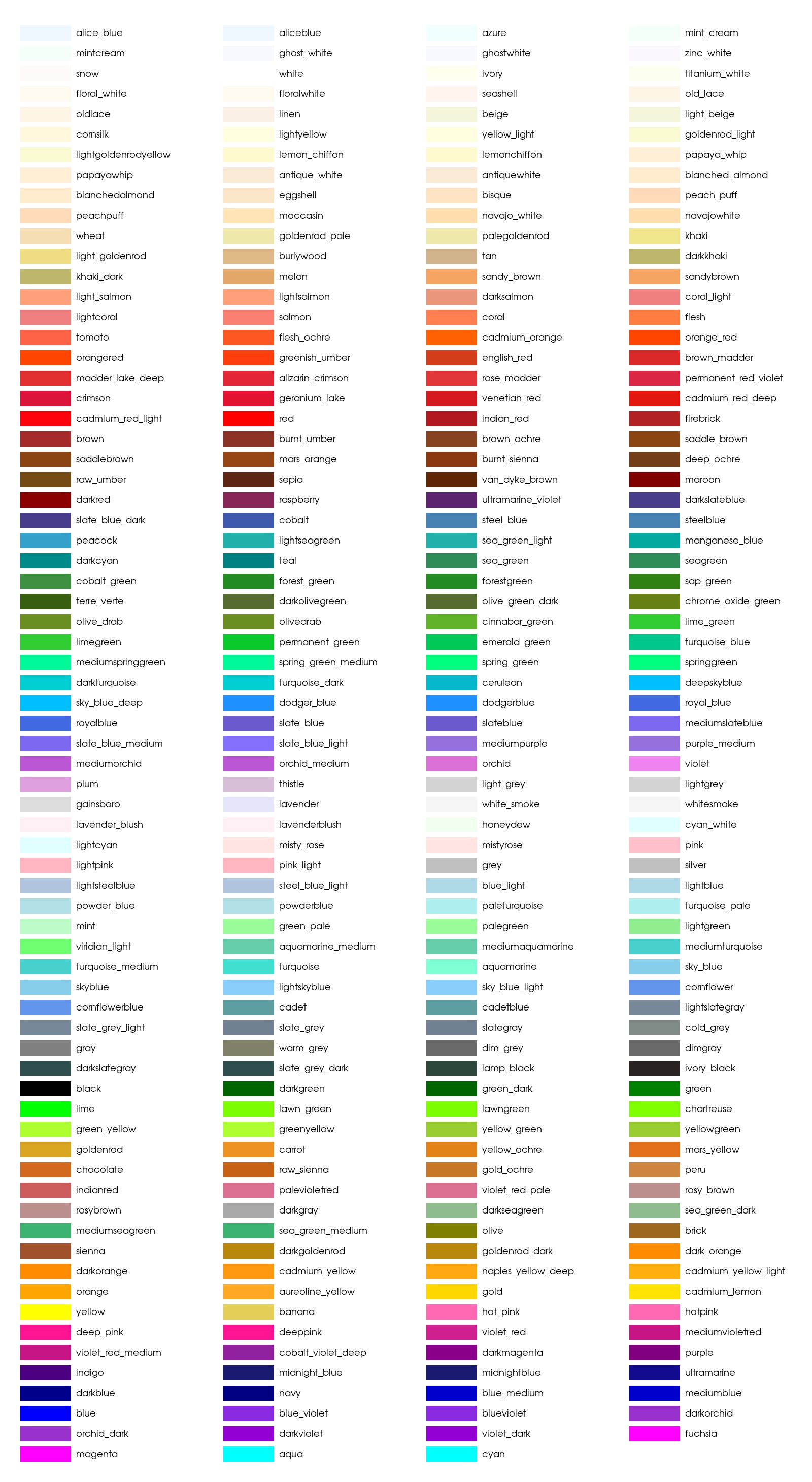
Colors ¶

All the colors related keywords in this treatment expect either a VTK named color or a hex color string (e.g. '#005A9C'). You can check the available named colors clicking in the images below.

Sorted alphabetically:
Sorted by similarity:

Warning

The availability of color names may vary depending on your VTK installation. To view the list of supported colors in your environment, you can run the following command

import vtk
vtk.vtkNamedColors().GetColorNames()

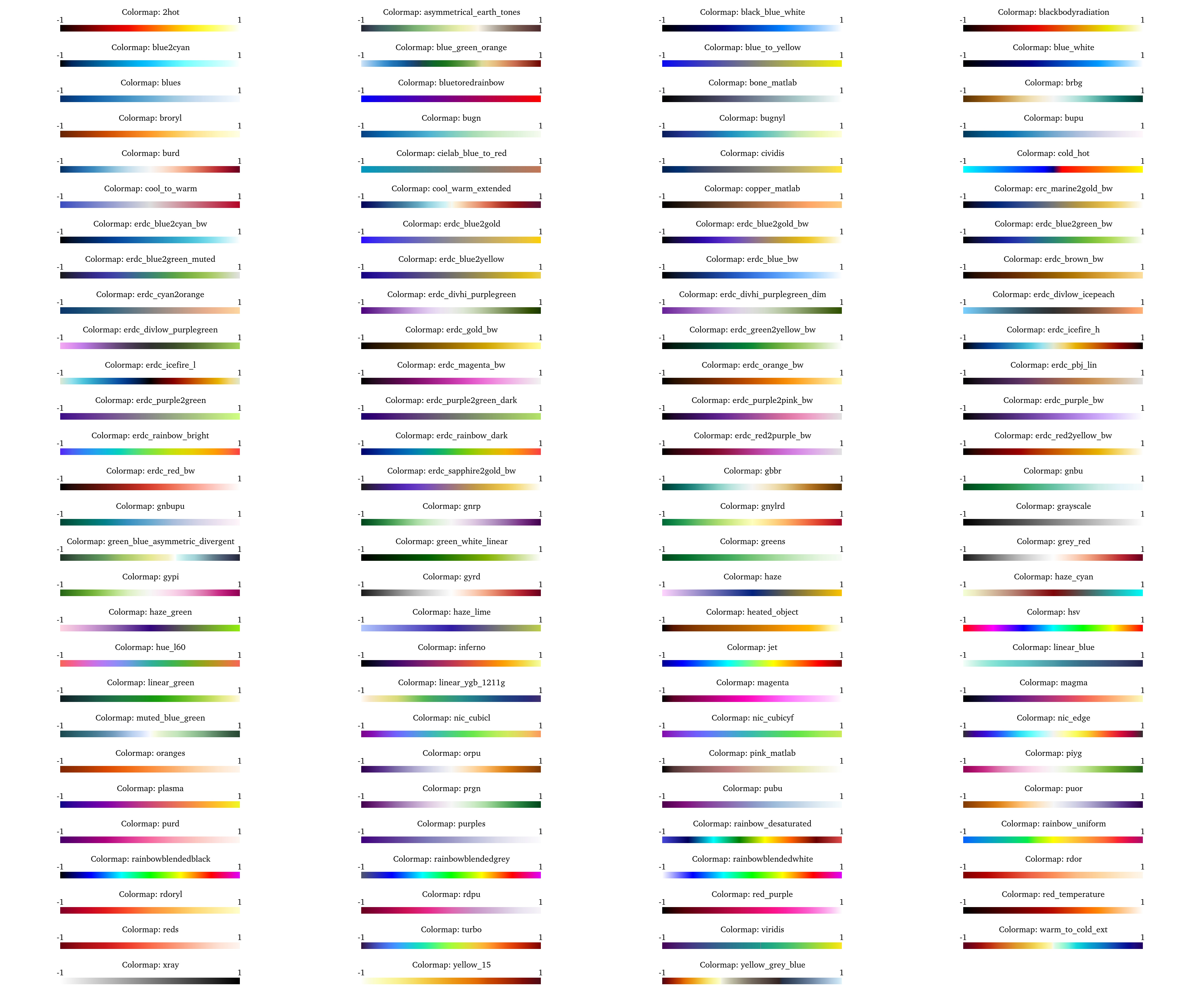
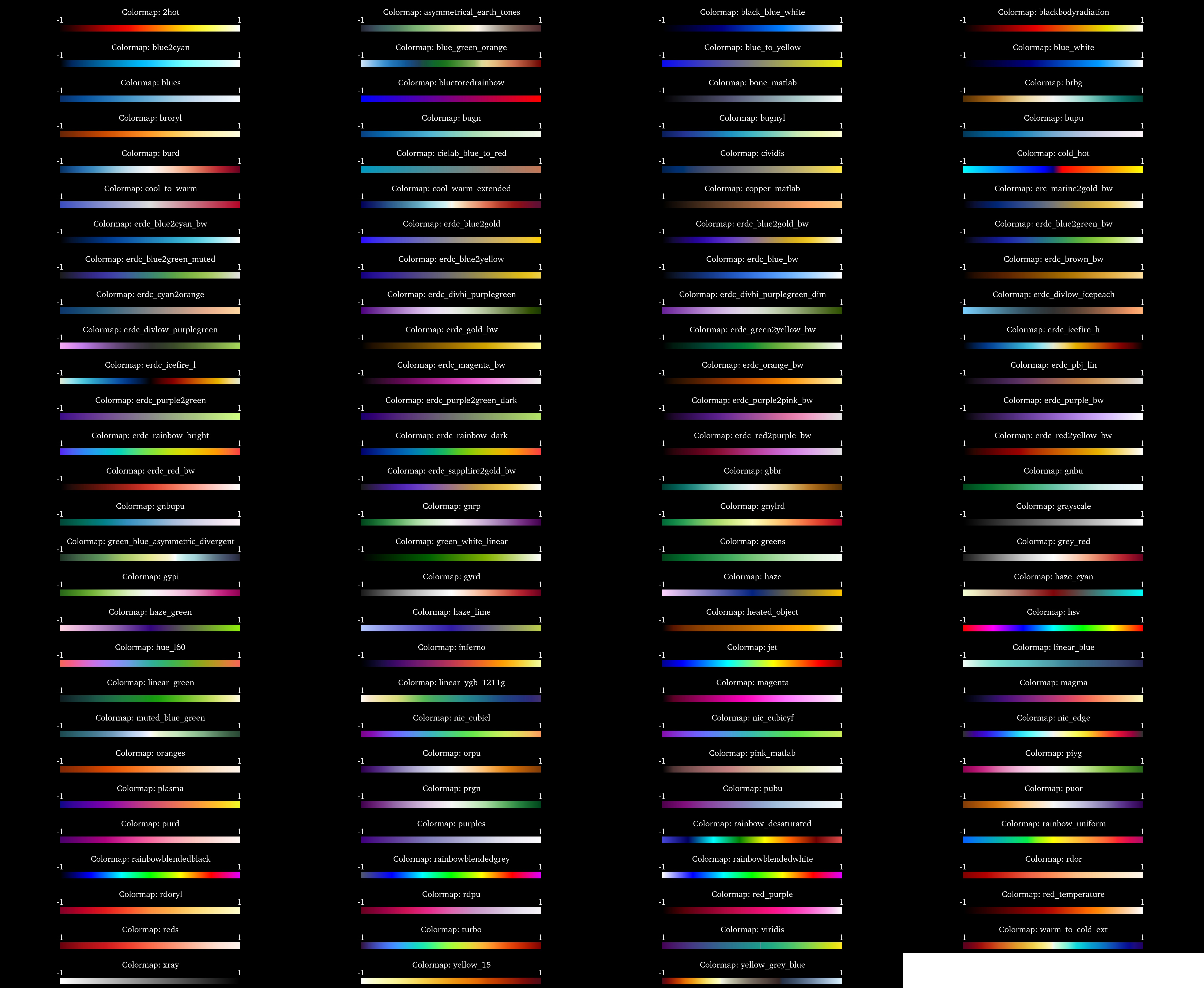
Colormaps ¶

Colormaps can be specified in two ways:

By selecting a predefined colormap
By constructing a custom colormap

Predefined Colormaps ¶

This treatment supports most of the colormaps available in ParaView. You can consult all available predefined colormaps using the images below:

With white background:
With black background:

Custom Colormaps ¶

Users can define their own colormaps by specifying a tuple of two elements using the colormap keyword.

The tuple must contain:

A list of colors that could be named of hex strings colors (see Colors). The colors will be equally spaced along the scalar value range.
A color space name that defines how interpolation between colors is performed.

The following color spaces are supported for interpolation:

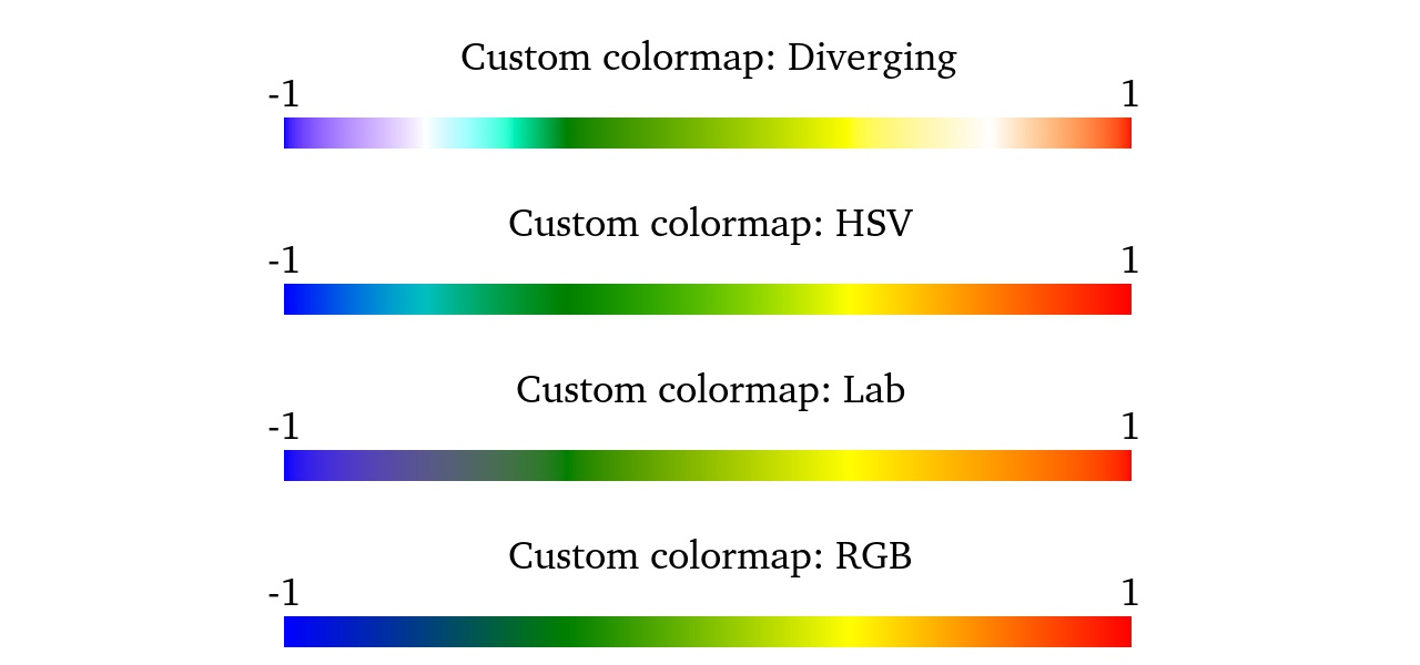
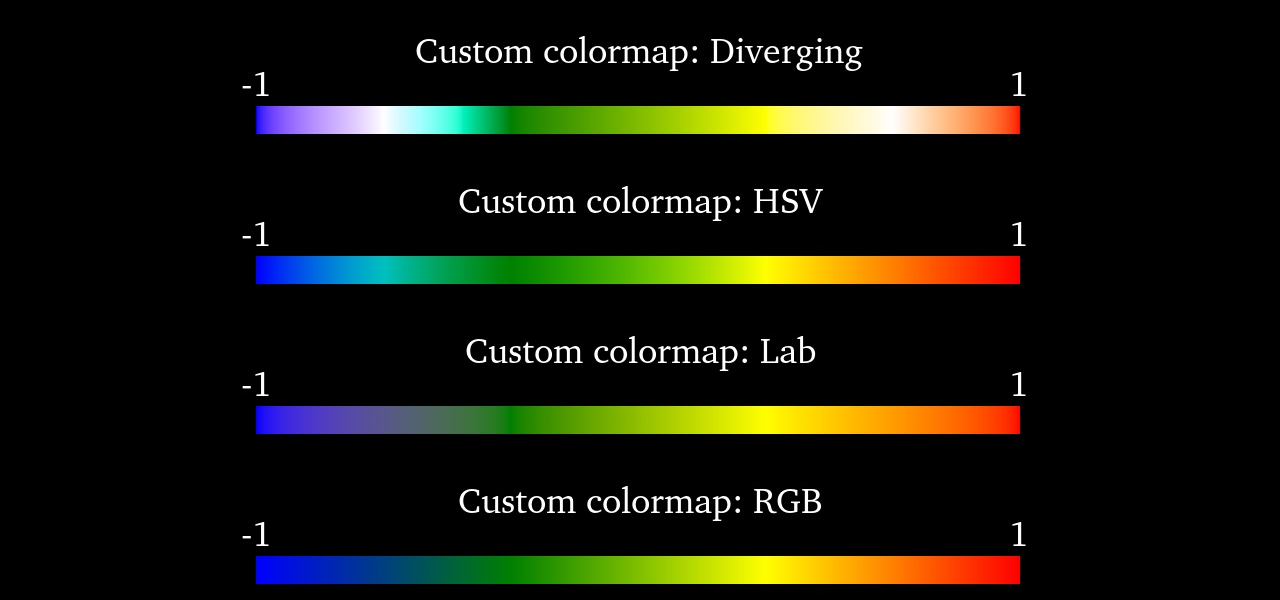
"RGB": Standard red-green-blue linear interpolation. Not perceptually uniform.
"HSV": Interpolation in hue-saturation-value space. Hue wrapping is enabled for smooth color transitions.
"Lab": Interpolation in the CIE L*a*b* color space. This space is perceptually uniform, meaning equal steps correspond to equal perceived changes in color.
"Diverging": Designed for diverging datasets (e.g., values around a central neutral point). Interpolates symmetrically between endpoints.

# Colormap going from Blue -> Green -> Yellow -> Red using a HSV color space
treatment['colormap'] = ( ['blue', 'green', '#FFFF00', 'red'], 'HSV' )

This creates a smooth, perceptually uniform gradient in Lab space.

Below you can find an example of the effect of the color space in a colormap of 4 colors: ['blue', 'green', 'yellow', 'red']

With white background:
With black background:

Colorbar labels ¶

The labels displayed on the colorbar are controlled by the 'colorbar_labels' keyword. This keyword accepts either a list of numeric values, special string values, or tuples for custom text labels.

Using Numeric Values ¶

You can provide a list of float values to specify exactly which values should appear on the colorbar. For example, the following sets the labels to 0.1, 0.3, 0.7, and 1.0:

treatment['colorbar_labels'] = [0.1, 0.3, 0.7, 1.0]

Using Special Values ¶

Two special string values are recognized: 'min' and 'max'. These automatically correspond to the minimum and maximum values of the colorbar range:

treatment['colorbar_labels'] = ['min', 0.1, 0.3, 0.7, 'max']

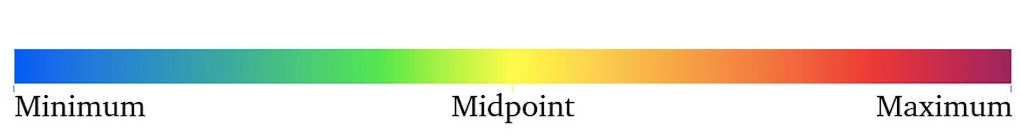
Adding Custom Text Labels ¶

You can also include custom text labels. To do this, provide a list of tuples, where each tuple consists of:

The location for the label (numeric value or 'min'/'max')
The text string to display

For example:

treatment['colorbar_labels'] = [('min', 'Minimum'), (0.5, 'Midpoint'), ('max', 'Maximum')]

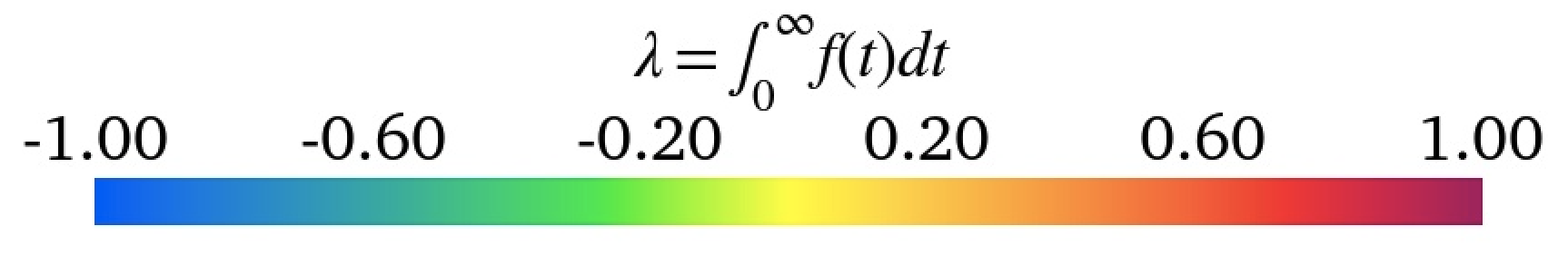
Using LaTeX expressions ¶

If your VTK installation supports LaTeX-style notation, you can enable it in this treatment by prefixing strings with r. For example, you can include LaTeX expressions in your colorbars like this:

treatment['colorbar_title'] = r'$\lambda = \int_0^{{\infty}} f(t) dt$'

This will generate the following colorbar:

$../../../../_images/latex.png$

You can check if your VTK installation supports LaTeX notation by doing:

import vtk
renderer = vtk.vtkMathTextFreeTypeTextRenderer()
print("MathText supported?", renderer.MathTextIsSupported())

Note

If you need to use curly brackets in your expression, you must escape them by doubling the brackets. For example, to render {\infty}, you should write it as {{\infty}}.

Font families ¶

VTK natively supports the following font families:

times:
arial:
courier:

Additionally, you can specify any of the font installed in your system (provided that VTK can read it). To use it you can use the fontname related keywords to specify a custom font family name. fontname takes as value the name of a font already installed in your system or the path to a custom font. If both, fontfamily and fontname are specified at the same time, fontname will take precedence.

To check the list of installed fonts readable by VTK, you can do:

import antares.utils.fonts
antares.utils.fonts.list_fonts()

Note

Using custom font families requires matplotlib to find the installed fonts in your system.

Warning

Mixing custom font families with LaTeX expressions does not work well because VTK uses a separate rendering backend for LaTeX-like math text which bypasses the normal font handling system. When math rendering is enabled, VTK relies only on the limited set of built-in font families (times, arial and courier) and ignores arbitrary custom fonts. Therefore, using fully custom font files with LaTeX expressions will silently fall back to the default math font, leading to inconsistent or unexpected results.

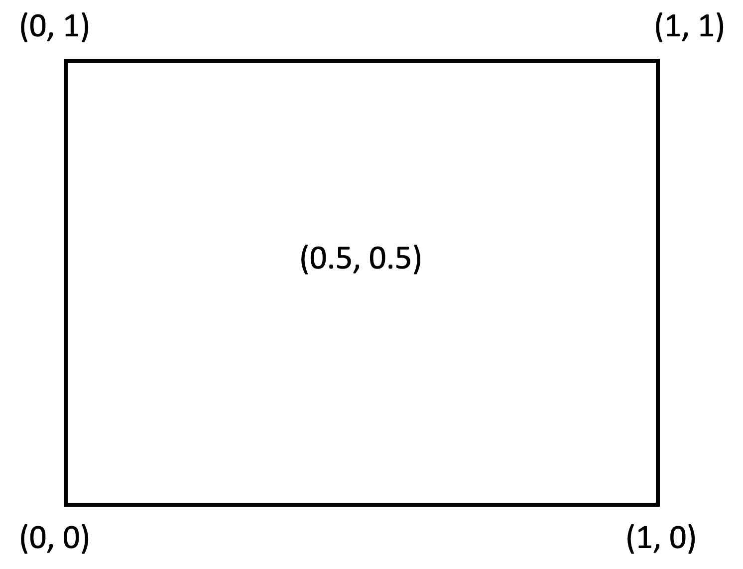
Relative coordinates ¶

The position of some objects (colorbars, text, images) can be specified by a pair of relative coordinates. The origin of the system is at the bottom left of the image an it corresponds to the coordinates (0, 0), and the top right corner of the image corresponds to (1, 1).

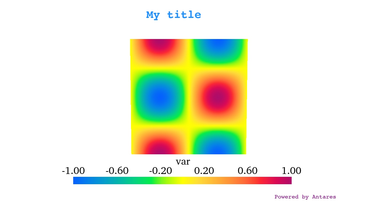
Inserting text ¶

If you want to insert custom text in the image, you need to use the texts keyword. This keyword accepts a list of dictionaries. Each dictionary specifies the text to be inserted as well as the text properties. The dictionary must be formatted as follow.

title = {
    'text': "My title", # Text to be inserted
    'position': [0.5, 0.9], # Text position in relative coordinates
    'fontsize': 40, # Font size (optional, default=36)
    'fontfamily': 'courier', # Font family (optional, default='times')
    'color': 'dodgerblue', # Font color (optional, default='black')
    'bold': True # If the text must be bold (optional, default=False)
    'fontname': None # Insert a custom font, overrides font family (optional, default=None)
}

footer = {
    'text': "Powered by Antares", # Text to be inserted
    'position': [0.9, 0.05], # Text position in relative coordinates
    'fontsize': 20, # Font size (optional, default=36)
    'fontfamily': 'courier', # Font family (optional, default='times')
    'color': 'purple', # Font color (optional, default='black')
    'bold': False # If the text must be bold (optional, default=False)
    'fontname': None # Insert a custom font, overrides font family (optional, default=None)
}

treatment['texts'] = [title, footer]

This will add a title and a footer to the image.

Warning

The text and position keys are mandatory

Inserting images ¶

If you want to insert custom images in the image, you need to use the images keyword. This keyword accepts a list of dictionaries. Each dictionary specifies the image to be inserted as well as the image properties. The dictionary must be formatted as follow.

mylogo = {
    'image': "cerfacs.jpeg", # path to image to be inserted
    'position': [0.7, 0.9], # image position in relative coordinates
    'scale': 0.5, # Shrink or enlarge the image by this factor(optional, default=1)
}

treatment['images'] = [mylogo]

This will add a logo near the top right corner

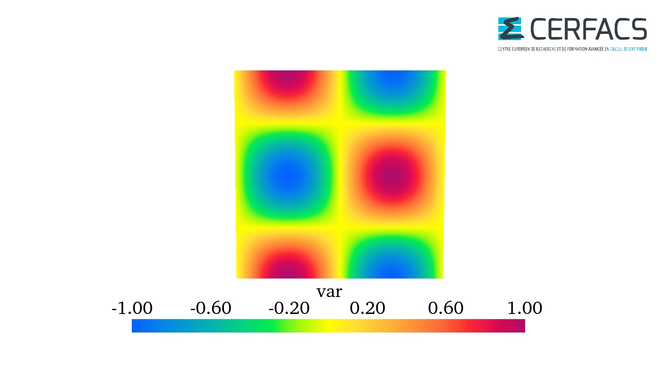
Warning

The image and position keys are mandatory

Camera control ¶

There are three ways to control the camera used for rendering:

Preset camera directions

You can specify one of the standard camera directions using the camera_direction keyword:
- X+ (positive X-axis view)
- X- (negative X-axis view)
- Y+ (positive Y-axis view)
- Y- (negative Y-axis view)
- Z+ (positive Z-axis view)
- Z- (negative Z-axis view)
- iso (Isometric 3D view)
These are simple shortcuts to orient the camera along the main Cartesian axes.
Manual camera parameters

For more fine-grained control, you can specify the camera parameters directly using the following keywords:
- camera_position
- camera_focal_point
- camera_zoom
- camera_view_up
- camera_angle
- camera_parallel_projection
If you do not know the exact values for these parameters, you can determine them interactively:
- Launch an interactive plot window, with show = True.
- Adjust the camera as desired.
- Press the c key.
- The current camera settings will be printed in the terminal.
- Copy and paste these values into your script using the above parameters.
Camera settings persistence

For saving and restoring camera states between sessions or executions, use the following options:
- camera_save_settings: The filename where the current camera settings will be saved whenever the user interacts with the window.
- camera_load_settings: The filename from which camera settings will be loaded.
If both parameters are set to the same filename, the camera settings will persist between runs, saving the last used camera state and reloading it automatically.

Jupyter integration ¶

The treatment can be integrated in Jupyter environments for both interactive and static visualizations. However, due to differences between JupyterLab and classic Jupyter Notebook, there are some important considerations and setup steps to ensure smooth functionality.

Interactive rendering is supported only inside JupyterLab. It produces an interactive widget that allows live manipulation of the visualization (zoom, rotate, pan).
In classic Jupyter Notebook or other non-widget environments, the rendering falls back to a static image , which is non-interactive.

To enable interactive rendering inside JupyterLab, you need to install the following Python packages with these exact versions:

ipywidgets==7.7.5
ipyvtk-simple==0.1.4
ipyvtklink==0.2.3
ipyevents==2.0.2
ipycanvas==0.13.3
ipykernel==6.29.5
jupyterlab==3.4.4

You can install these packages via pip with:

pip install ipywidgets==7.7.5 ipyvtk-simple==0.1.4 ipyvtklink==0.2.3 ipyevents==2.0.2 ipycanvas==0.13.3 ipykernel==6.29.5 jupyterlab==3.4.4

After installing the required Python packages, the corresponding JupyterLab extensions need to be enabled to ensure full interactivity in JupyterLab. This can typically be done using the following commands:

jupyter labextension install @jupyter-widgets/jupyterlab-manager@3.1.11
jupyter labextension install ipycanvas
jupyter labextension install ipyevents

To enable the correct rendering mode, you must set the keyword 'jupyter' to True

To correctly display the rendered output in Jupyter, retrieve the render object returned by the treatment’s execute method and wrap it in an interactive widget using ipyvtklink.

from ipyvtklink.viewer import ViewInteractiveWidget

render = treatment.execute()
widget = ViewInteractiveWidget(render)
widget  # Important: This line must be the last expression in the notebook cell
        # to trigger the display of the interactive render window.

Note

When using jupyter only the first instant is rendered.

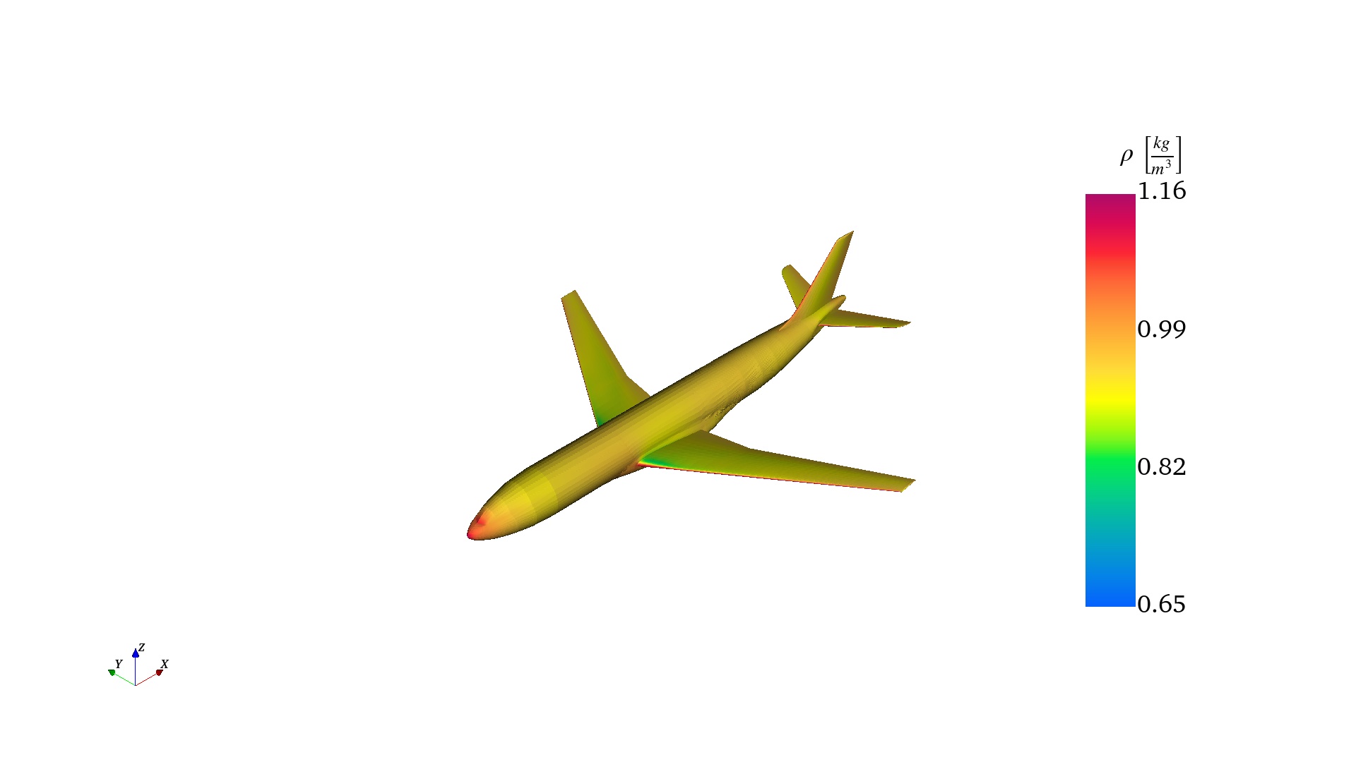
Example 1: Plot single base ¶

The following example shows how to plot a single base with a custom isometric view:

import antares
import os

data_folder = os.path.join('..', 'data', 'AIRCRAFT',)
output_folder = os.path.join('.', 'OUTPUT', 'plotbases')
os.makedirs(output_folder, exist_ok=True)

reader = antares.Reader('hdf_antares')
reader['filename'] = os.path.join(data_folder, 'skin.h5')
skin = reader.read()

# Show base
plot = antares.Treatment('plotbases')
plot['bases'] = skin
plot['color_by'] = 'ro'
plot['colorbar_title'] = r'$\rho$ $\left[\frac{{kg}}{{m^3}}\right]$ '
plot['colorbar_nb_labels'] = 4
plot['camera_direction'] = [-1, -1, 1]
plot['show'] = False # Set to True to open interactive window
plot['output_file'] = os.path.join(output_folder, 'aircraft_density.jpeg')
plot['figsize'] = [1920, 1080] # full HD resolution

plot.execute()

../../../../_images/aircraft_density.jpeg

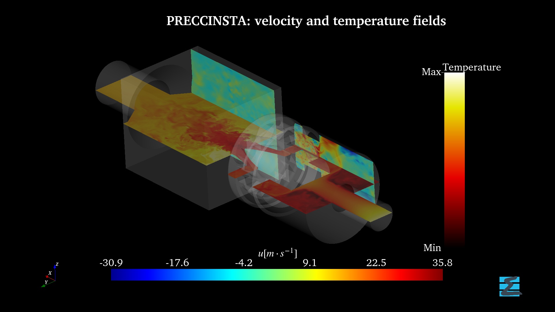
Example 2: Plot multiple bases ¶

The following example shows how to plot different bases with different variables. The geometry corresponds to the PRECCINSTA burner. The geometry boundaries are shown in a transparent gray color. Two different cuts are shown: The temperature field and the axial velocity field with two different colormaps. Additionally, a title and the CERFACS logo are added to the image, and the image background is set to black.

import antares
import os

data_folder = os.path.join('..', 'data', 'PRECCINSTA_VISU')
output_folder = os.path.join('.', 'OUTPUT', 'plotbases')
os.makedirs(output_folder, exist_ok=True)

# Read the burner's boundaries
# ----------------------------
geom = antares.io.Read(
    format='hdf_antares',
    filename=os.path.join(data_folder,"preccinsta.h5"),
  )

geom.attrs['plotbases'] = {
    'color_by': 'zones', # Plot by zones
    'zone_colors': 'white', # All zones are gray
    'colorbar': False, # Do not show the colorbar
    'transparency': 0.85, # 85% transparency
  }

# Read a cut XY
# -------------
cut_xy = antares.io.Read(
    format='hdf_cgns',
    filename=os.path.join(data_folder, 'slice_xy.cgns'),
  )
cut_xy.attrs['plotbases'] = {
    'color_by': 't', # Plot the t variable (temperature)
    'colorbar_labelformat': '%.2f', # Label's float notation with 2 decimals
    'colorbar_title': "Temperature", # Colorbar title
    'colormap': 'blackbodyradiation', # Black-red colormap
    'colorbar_labels': [('min', 'Min'), ('max', 'Max')], # Add custom label text
}


# Read a cut XZ
# -------------
cut_xz = antares.io.Read(
    format='hdf_cgns',
    filename=os.path.join(data_folder, 'slice_xz.cgns'),
  )

cut_xz.attrs['plotbases'] = {
    'color_by': 'u', # Plot the axia velocity
    'colorbar_horizontal': True, # Show a horizontal colorbar
    'colorbar_title': r'$u [m \cdot s^{{-1}}]$', # Colobar title using latex
    'colorbar_labelformat': '%.1f', # Label's in float notation with one decimal
    'colormap': 'jet', # Blue-red colormap
}

# Add a title in the top middle part of the window
# ------------------------------------------------
title = {
    'text': "PRECCINSTA: velocity and temperature fields",
    'position': (0.3, 0.95),
    'fontsize': 46,
    'bold': True,
    'color': 'white'
  }

# Add a logo in the bottom right corner
# -------------------------------------
logo = {
    'image': os.path.join(data_folder, 'cerfacs_logo.png'),
    'position': [0.9, 0.05],
    'scale': 0.25,
  }

# Show base with text and title and with a specific camera position
plot = antares.Treatment('plotbases')
plot['bases'] = [geom, cut_xz, cut_xy,]
plot['color_by'] = 'in_attr'

plot['colorbar_title_fontcolor'] = 'white'
plot['colorbar_ticks_fontcolor'] = 'white'

plot['texts'] = [title]
plot['images'] = [logo]

plot['axes_fontcolor'] = 'white'

plot['camera_position'] = (-10.49, 8.46, 7.01)
plot['camera_focal_point'] = (-0.0234, -0.016, -0.00421)
plot['camera_view_up'] = (0.324, -0.33, 0.88)
plot['camera_zoom'] = 1.0
plot['camera_angle'] = 1.0
plot['background_color'] = 'black'

plot['show'] = False # Set to True to open interactive window
plot['figsize'] = [1920, 1080]
plot['output_file'] = os.path.join(output_folder, 'preccinsta_dark.jpeg')
plot.execute()

../../../../_images/preccinsta_dark.jpeg

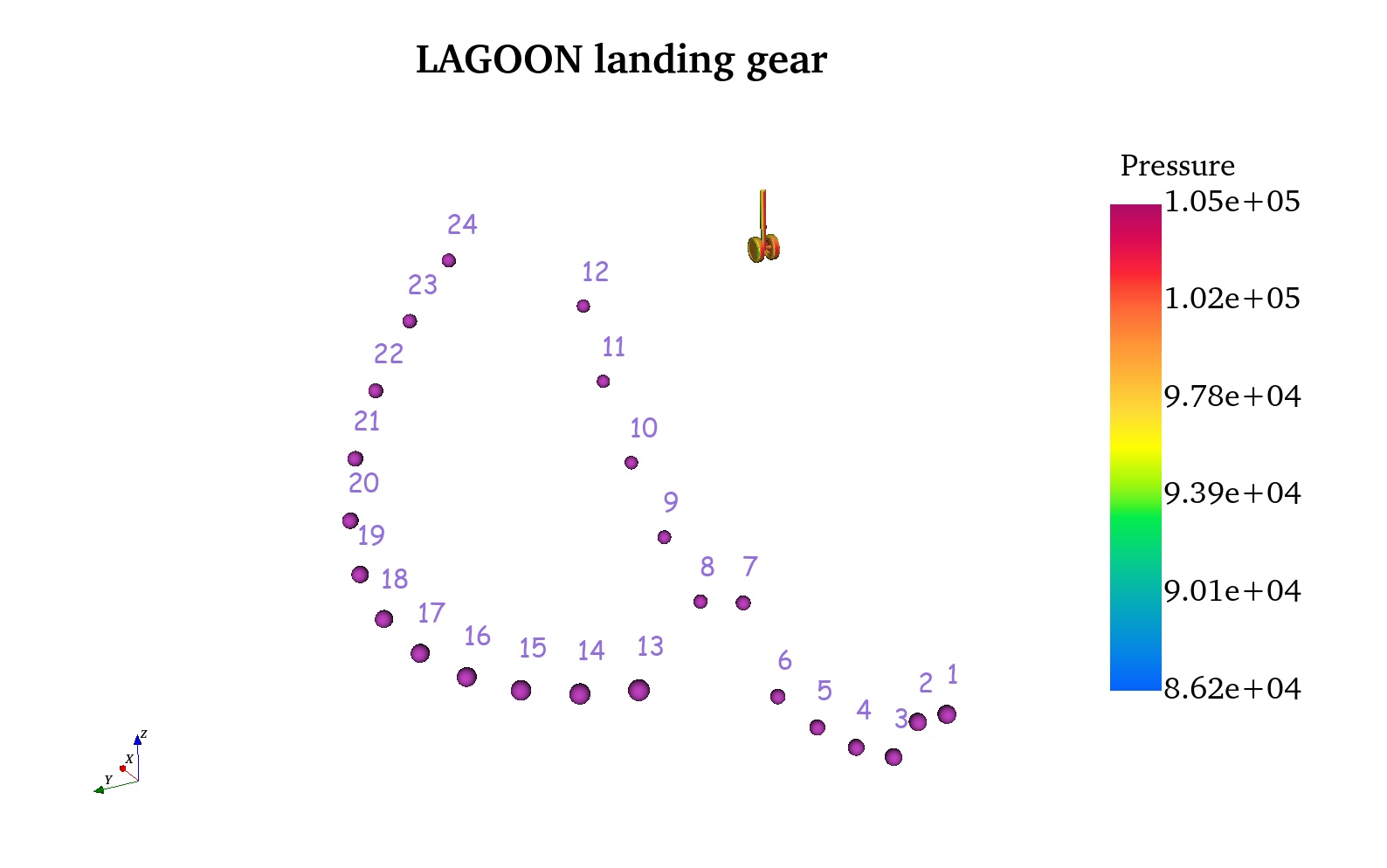
Example 3: Plot single bases and list of points.¶

The following example demonstrates how to visualize a single geometry (the LAGOON landing gear) alongside a set of points representing microphone positions used for aeroacoustic analysis based on the Ffowcs Williams–Hawkings analogy. The LAGOON geometry is color-mapped by pressure, while the microphones are colored using a hex color strings with labels drawn next to them. Finally, camera properties are restored from a configuration file (camera.txt) previously generated by running the same script with the parameter 'camera_save_settings'.

import antares
import os

data_folder = os.path.join('..', 'data', 'LAGOON')
output_folder = os.path.join('.', 'OUTPUT', 'plotbases')
os.makedirs(output_folder, exist_ok=True)

# Read the lagoon simulation
# --------------------------
base = antares.io.Read(
    format='hdf_antares',
    filename=os.path.join(data_folder,"lagoon.h5"),
  )

base.attrs['plotbases'] = {
    'color_by': 'scalarPressure', # Plot by pressure
    'colorbar_title': 'Pressure',
    'colorbar_labelformat': '%.2e', # Labels are shown in scientific notation with 2 decimals
}

# Read microphones
# ----------------
micros = antares.io.Read(
    format='column',
    filename=os.path.join(data_folder, 'micros.txt')
  )

micros.attrs['plotbases'] = {
    'color_by': 'zones',
    'zone_colors': '#BF40BF', # Probes are colored in dark purple
    'colorbar': False,
    'point_radius': 0.1,
    'point_show_labels': True, # Show probe labels
    'point_label_offset': [0, 0, 0.3], # labels are offset by 0.3 in the Z direction with respect to the probe's position
    'point_label_color': 'mediumpurple', # Label color
    'point_label_fontsize': 30,
    'point_label_fontname': 'Comic Sans MS', # Comment if you don't have this font installed in you system
    }

# Add a title in the top middle part of the window
# ------------------------------------------------
title = {
    'text': "LAGOON landing gear",
    'position': (0.3, 0.95),
    'fontsize': 46,
    'bold': True,
  }

# Show base with text and title and with a specific camera position
plot = antares.Treatment('plotbases')
plot['bases'] = [base, micros]
plot['color_by'] = 'in_attr'

plot['texts'] = [title]

plot['point_labels'] = 'base'
# If 'show' is set to true, any change in the camera position will be
# saved and restored next time the script is executed.
plot['camera_save_settings'] = os.path.join(data_folder, 'camera.txt')
plot['camera_load_settings'] = os.path.join(data_folder, 'camera.txt')


plot['show'] = False # Set to True to open interactive window
plot['figsize'] = os.path.join(data_folder, 'camera.txt')
plot['output_file'] = os.path.join(output_folder, 'lagoon.jpeg')
plot.execute()